Class outline
Class 1:
Get syllabus, go over it, pair programming, class web pages,
assignments page, submitting in Blackboard
Get you picture taken. Make sure you can log in.
!!! Flash
Drives!
See Assignment in Schedule for before next class.
What is Computer Science centers on algorithms:
unambiguous, step by step
instructions for how to accomplish a particular task in a finite amount
of time. There are many aspects, and college
introductions have handled things differently over time:
- Historically started with usually several heavy
programming
courses before anything else, giving little inital idea what you were
getting into!
- Then there was a reaction to
breadth-first, essentially no
programming. This is partly because in the past popular
languages
had a steep learning curve. Instead of
much programming in a
real computer language,
breadth-first courses have brought algorithms written in
English
to a central place.
- That brings us to the present
with this course.
Programming
is important, and now there is an excellent recent
language Python: extremely simple to learn and
understand
(close to English) and very powerful -- why do much in
English
outlines when with about as much work you
can demonstrate things on the computer using Python? Plus,
even
beginners can write programs to simplify their own personal tasks.
Hence we spend a fair amount of our time on algorithms
actually
working with Python. We still keep the idea that Computer
Science
is much more than programming, and look at history and social and
ethical implications. We dig down into the guts of a computer
below what we see from the high-level language Python, to
machine
language and assembler code, and to the hardware underneath.
We
look beyond Python to application areas like graphics and web servers.
For the programming in Python, we use Zelle.
For
most of the
other topics, we use Decker/Hirshfield. The two come close
together when DH discusses web pages. We will simplify the
web
page creation, relying on recent free software that makes writing web
pages be basically using a special word processor. Like DH,
we
want interaction with our web pages. There are two possible
approaches, both
using web pages with forms on them: DH chooses interaction
restricted to the
users
machine, with no memory between sessions, no interaction with
other users,
using a specialized language called Javascript, just for use
in browsers. Another approach is to place
intelligence on the
web server, where we have a choice of programming languages, and we
choose Python, of course!
We are not alone in choosing Python: Much of the
control of
Google is by Python, as is much of the administration of Unix.
(Microsoft has not adopted Python, since it does not own this
free language, but Python is freely available for Windows, modern Macs,
Linux ....)
Make pairs, conveying information visually: Indicate if you
live
on campus,
are a
night person, have time after class, have time right before class, are
flexible on weekends....?
Examples of final Python projects
Wrote
text based program, graphics
programs, web based programs.
People had complete freedom in their final project.
A web one http://webpages.cs.luc.edu/~kechampagne/astro.html
and I will demostrate a couple of graphical ones. All but one
are by people without previous programming experience.
Who
using what resources: These labs, other IS labs - (get a
Flash Drive!), own computer with Windows? Mac? Linux?Starting
Python in the lab. See Lab
1.
Class 2
little of
Zelle
Sign under your picture: Nick name or first name,
follwed by last name.
Mock quizzes (each is one
question).
1. Briefly compare
and contrast: algorithm and program
2.
What does the following first program line mean
to the Python
interpreter?
# File: chaos.py
Quiz
procedures.
Questions on Zelle reading.
- what stood out for you as important,
meaningful or hard?
- type in program and computer
directly
execute what you typed?
- syntax templates make
sense?
Pair Programming partners: Ask to help people
choose: Free before class; free after class; free and on
campus weekday evenings; flexible on campus weekends; + ?
More
of Lab 1. Starting Idle for
Python.
Z
ch 2
Zelle questions
note appendix A, p 469!
Intro to Program 1
Intro to idle files, work in class easy
input/process/output pattern. Input a number, output with the
square. Note the input
glitch in idle!
commenting out a block of lines
with alt-3 or the edit menu
Lab 2
Class 3
ch 3 Zelle - range examples
loops
in shell -
- in idle indent automatically, hit
<enter> twice to end
range in for loop as replacement for explicit sequence
vary future value: print year, by year,
with label 1, 2, 3, ....
Lab
3 Task 1
Class 4
example file
loopIdea.py
Do
rest of Lab 3
Class 5 History
Themes
- Methods
and pace of improvements
- Layers added vs. improvements in implementation
- Interplay between hardware, software, theory, and
applications imagined
- Abstract ideas that make sense with very different
hardware and implementation
- Interfaces and industrial standards
- Machines
doing what humans used to do
Elaboration on Ada
Lovelace: http://en.wikipedia.org/wiki/Ada_Lovelace
More
on Lab 3
Back to Zellech 4 string stuff on
slices
s =
"computer"
To refer to a single element with a
substript, it is easier to think of the data and indices as lined up:
index from left 0
1 2 3 4 5
6 7
data sequence
c o m p u
t e r
index from
right -8 -7 -6 -5 -4
-3 -2 -1
s[2] # 'm'
s[-2]
# 'e'
For slices it is
easier to think of indices between data elements:
index from left 0
1 2 3 4 5
6 7 8
data | c | o | m
| p | u | t | e | r |
index from right -8
-7 -6 -5 -4 -3
-2 -1
s[2:4]
# 'mp'
If you use the same diagram to refer to a
single subscript: the data comes to the right of the
subscript
Contrast:
when using a single
subscript, the index must give an actual location in the
string;
but in slices, references to nonexistent
elements are just ignored.
s[10] # error
s[2:10]
# 'mputer'
s[4:2] # '' (empty string)
Programming
patterns so far:
- input/process/output
- accumulator
for iterative changes: initialize
accumulator, update accumulator for a sequence of data in a loop
Do
Lab 4 tasks 1-3
Class 6, Discussion of
String
operations
Numerical programming use all the most common operations and
symbols. In string programming, there are again fairly common
operations, but the syntax is new, and you need to get used to what
basic operations are available: see table page 96!
Play
with these in the shell - - the worst that happens is that you get an
error message back!
Example: Write a program to input a string and print it in
upper case.
Note the input
function is not what you want - - what do you use?
s = raw_input("Enter a line: ")
print string.upper(s)
Again, the early syntax in 4.1 used for strings works for
any sequence,
including a sequence of strings or anything.
Program: Read in a string and print out one word
to a line.
One approach:
s = raw_input("Enter a line: ")
words = string.split(s)
for word in words:
print word
Another approach: everything that goes to the
screen is
characters, including invisible parts like blanks and newlines.
printing word one to a line means:
word 1 newline word 2 newline ...
i.e. words with newlines between - - that suggests the join
method
s = raw_input("Enter a line: ")
words = string.split(s)
print string.join(words, '\n')
Rest of Lab 4
Class 7
See the Review for Exam 1 -- link
on the course home page
Selected text
solutions on web under Solutions link - - need
id/password - - get it in class or from Blackboard Class Content page.
CAUTION:
The answers
serve almost no purpose if you look first and then work on them or
never work on them. Reading is WAY different than writing!!!
If you are having trouble, resist the urge to look at the
answers. The significance of the answers is not their actual
text
but the mental process coming up with them!!!
Learning
in English: read and understand, write,
practice writing!
Learning in programming: read and understand, write, practice
writing!
Difference: Priog languages picky about syntax.
hastle
getting it right, but good to get direct feedback (On more complicated
problems it is still an enormous issue to be sure you are right in all
cases.)
formating use -
Z 106. later files - p114
Play with formatting:
See example code
stringFormat.py.
Notes on the
syntax summary:
- Width is the
minimum width -- extra space is taken if needed.
- Precision
(if present) must be preceded by the decimal point.
- When
more than one data element is to be formatted
and embedded in the format string, the values are separated by commas
and enclosed in parentheses. This is a another kind of
sequence,
a variant on a list called a tuple.
- The
precedence of operators is always the same, whatever the type of the
operands. Note that in the showWidth function, there are
parentheses around "x"*n. They are not making a tuple --
there is
only one string expression intended as the data. See what
happens
when you remove the parentheses. Explain this in terms of the
precedence of the operators % and *. (The % operator is
related
to division and has the same precedence as division.)
Do Lab 5 task 1
Strings
and
numbers: chr, ord
for ch in "abcABC123!":
print ch, ord(ch)
for n in range(32, 60):
print n, chr(n)
For Each:
Above are
examples of "for each" loops: do something for each element
of a
sequence. In the simplest situations, like above, the results
from processing each element are basically independent -- what happened
on the previous one odes not affect the next one.
It
is very important to understand the power of these ideas with
loops and be able to apply them: If you know how to write
instructions for how to do something with one piece of data, you can
always process a sequence of such data in a loop. When
solving a
problem for independent handling of a sequence of data values, you can
always split the problem into two parts:
- How
to handle one single case
- How to repeat in a
loop
In
more complicated situations the results accumulate somehow, with each
time through the loop making incremental changes to a result (or
possibly several results). This accumulator pattern is also
very
important.
Counting
through a sequence
Often
you want to process each element of a sequence and keep a count.
For instance to help you associate the right index number
with
each character in a string, we could write a loop to put the index of
each character and the character itself on a line. We will
want a
loop. Since we want to print two pieces of data, index and
character, we have several choices:
A.
for each index of a character in the sequence
or
B. for
each character in the sequence
A.
Given a string s, how do you loop through each index in the
string?
Inside the loop, given the index, how do you get the
corresponing character?
B. How do you loop
through each character in a string directly?
See the
example stringIndex.py for the details.
(Coding
each of these is instructive. Also there is a more direct
way, that is specific to Python: if you want to get
deeper
into Python see the enumerate
function in the Python documentation.)
Class 8
Files
With
files we will often have "for each" loops: either for each
character or each line or each word.
Rest of Lab 5
Introduce Program 2.
Strings and files as Objects
Class 9
Exam 1 ch 1 of DH, ch 1-4 of
Zelle, stopping before filesClass 10
From
examples - graphics.py to program directory -- new version, updated for
today!
updated zelle_code under password
Display graphics? Mention logic that we are using a
restricted version
Point out Graphics web pages under
notes
objects, common features, clone, aliases,
triangle.py
Lab 6
polygon#.py 0-1
polygon#.py 2-3
Lab 7
Class 11
Entry,
Fahrenheit example
Lab 8
Class
12
Start Decisions
ifExamples.py Lab 9
Class 13
While
loops: counting loop
see examples: whileCount.py
Lab 10Class
14
interactive loops, sentinal loops example: makeList.py
graphics
example: polygon5.py
new hw 4
loop and nested if: remove blank lines
from a file -- complete example: filterEmptyLines.py
Class 15
list of ints to printed
pairs
coord = [10, 20, 5, 3, 30, 35, 40, 42]
print
a list of coordinates in pairs (10, 20), (5, 3), (30, 35), (40,42)
look
in slightly greater generality:
(s[0], s[1]), (s[2]],
s[3]), (s[4], s[5]), (s[6], s[7])
want pairs
0, 1
2,
3
4, 5
6, 7
??
process 2
each time:
by twos
for i in range(0, len(coord),
2):
how get 2nd of pair?
If i is
0, 2, 4 or 6,
what is
1, 3, 5, or 7 ?
string of ints to printed
pairs
moreLoops.py
make card deck +
random.shuffle(seq)
nested
loops, play computer
testBool.py
other
types converted to Boolean
Lab
11
Class 16
review materials for exam 2
functions
print string triangle for 'Bye!'
B
By
Bye
Bye!
print word triangle for any s
return String for triangle
isBetween(x, end1, end2)
distance(point1, point2)
makeCircle(center, ptOnCircle)
Lab 12
Lab 13
Class
17
exam 2
Class 18
Writing Web
pages, reading CGI scripts ( see
web pages)
Class 19
Web forms,
writing CGI scripts Program 5 introduction - Blackboard
assignment mechanism
Class 20
Finsih
writing your own dynamics web pages and CGI scripts
Class
21
mutable objects: mutable.py
New Assignment submission in Blackboard
use
DH 240-250
ch
6 in AE
place value - powers of 10, base 10
4072
= 4*103 + 0*102 + 7*101
+ 2
need symbols for the numbers less than ten (0-9)
think
of 4072 as a number. The symbolism is a numeral
representing a number.
Another representation could be a
pile of 4072 counters
or use a different base,
in particular the simplest one, and the one on which computers are
based:
binary use powers of 2 and two symbols 0, 1: base 2
I
will use a subscript to indicate the different base
110112
means in normal arithmetic:
1*24 + 1*23 +
0*22
+ 1*21 + 1
= 16 + 8 + 2 + 1 = 2710. (add up
powers of 2 where there is a 1)
shorthand for
base 2
24 23 22 21 20
16 8
4 2 1
1
1 0 1 1
again ad up the powers where there is a 1 in the numeral.
= 16 + 8 + 2 + 1 = 2710. (add up
powers of 2 where there is a 1)
bin To Decimal: done by Python. Try and look at the popup
window in the Python shell:
int('11011'
note the
second optional parameter, the base. Finish as
int('11011',
2)
see the correct answer.
The other
way: recovering the place values from an integer:
Suppose
we have an unknown int which is represented as a 4
digit
decimal. How could we recover the digits by doing simple
arithmetic? A bit of algebra can show us the genral approach:
For the algebra we need names for the 4 digits,
say p, q, r,
s, then we have
x = p*103 + q*102 + r*101
+ s
Note all but the last term are divisible by 10, so
s = x % 10
done with s, now let
x = x/10 = p*102 + q*101
+ r
same trick!
r = x % 10
Let
x = x/10 = p*101 + q
q = x % 10
Let
x = x/10 = p
p = x % 10
(To illustrate the general algorithm) Let
x = x/10 = 0 - - done
general:
def decimal(i):
"return a string of decimal digits reprsenting the nonnegative integer
i."
if i == 0:
return "0"
numeral = ""
while i != 0:
digit = i % 10
numeral = str(digit) + numeral # add next digit on the LEFT
i = i/10
return numeral
decimal
To Bin: same idea as for digits of
unknown number,
but base is 2, not 10:
def toBinary(x):
if x is 0:
return "0"
ans = ""
while x != 0:
digit = x % 2
ans = str(digit) + ans
x = x/2
return ans
Binary is verbose!: Compact it: convert
each 4 bits
to a single character:
Problem: Run out of normal digits: then start with letters,
so 10->A, 11->B, 12->C, 13->D,
14->E, 15->F
Bin to Hex
10111100
1011
1100 split in 4;s from the right
8+2+1
8+4 convert groups of 4 from binary
11
12
decimal results
B
C
convert to hexadecimal digits
BC
1011110011
(= 001001110011
but NOT 100111001100)
10
1111
0011 split in 4;s from the right
2
8+4+2+1 2+1
convert groups of 4 from binary
2
15
3
decimal results
2
F
3
convert to hexadecimal digits
2F3
Hex
to Bin
2F3
2
F
3
2
15
3
decimal
0010 1111
0011 binary, padded to 4 bits
001011110011
binary together
1011110011 binary together, shortened
see
bases.py
octal for Linux - permissions
3bit groups for
rwx use base 8
chmod 711 public_html
711
octal -- groups of three bits
7
1 1
111
001 001
rwx rwx rwx
111 001
001
rwx --x --x
Can do
hexadecimal and octal in format strings in Python:
formats %x %o
lab catchup
Class
22
Pip Assember
As we will see
more in Chapter 7, the state inside a computer is usually electrical,
and the
most dependable system uses voltages, either high or 0 (grounded) .
This means two
possibilities. This is a bit
of information, the smallest possible amount. We will
arbitrarily refer to the two states
as 0 and 1.
Computers have a Central
Processing Unit (CPU) connected by wires to a memory unit.
Operations
take place inside the CPU, with some data maybe transfered in from
memory or sent back to memory (and also external devices, though we
will skip that part in our simple model).
Like in a
Python list, memory is referenced by integer locations, 0,
1, 2, .... There are several design decisions: one
is how much data
to put in a single memory cell that can be individually referenced.
A
common unit is a byte = 8 bits. Pip uses a byte.
While a bit has two possible
states, a
byte has 28 = 256 states. Another
choice is how big to
allow memory to be. So that one byte can used to refer to any
cell
in memory, we will assume memory consists of no more than 256 cells.
Von
Neumann's concept was the encode the instructions as a form of data in
the computer. That means they must be a sequence of 0's and
1's, like
00010100 00000100
I
introduce the space in the middle only to delineate individual bytes.
Since accessing memory is slower than internal
operations in the CPU, all CPU's have places for special data to be
stored inside of them. One is an Instruction Pointer (IP),
saying where in memory the next instruction starts. CPU's
also have one or more fast temorary data storage locations.
In AE's simple example there is a single such location,
called the Accumulator or Acc for short, that holds a byte of
information, just like a memory cell.
Pip
Assembler Simulator
For a simple conceptual view, look at the
Pip Assembler simulator in the web examples.
Download
example files pipGUI.py, pipText.py, pip.py, pipHelp.py, hexBin.py.
It will really help to have a flash drive to keep all these
files on! All files are included in pipFiles.zip.While
you ar at it, download sample program
files (also in the zip archive):
simple.bin, simple.asm,
arith.asm, sum2n.asm, ifElse.asm
Run
pipGUI.py. You will see a graphical Window. Click
on the button that says BINARY, to see its 'native' state.
The
state of the simulated computer is shown in the CPU (lower left) with
its accumulator (Acc) and Instruction Pointer (IP). The
middle blue and right yellow blocks display memory.
First
focus on the big middle blue rectangle labeled CODE.
In Pip instruction code is placed at the
beginning of memory. Each instruction takes up two bytes, so
for convenience bytes are shown in pairs down the right
portion of the main blue rectangle. We will need to keep
track of the locations of these instructions, so the left column in the
blue rectangle shows the address (in decimal) of the
beginning of each instruction. Beside the decimal address
label is the same address in binary. Because each instruction
is two bytes, the address labels advance by 2's.
Now look at
the right yellow rectangle labeled DATA. For simpicity of
display, we arbitrarily assume that the data for program variables is
stored in the second half of memory, starting at address 128.
Each individual byte is a separate piece of data, so we show
only one per line, at the right. For our simple programs we
will never need more than 8 variables, so only eight locations are
displayed. As in the code section, address labels in decimal
and binary are shown.The remaining parts of the display are
for controlling the simulator. They do not correspond to
parts of Pip. The left column of buttons and text boxes is
labeled COMMANDS. You should have already clicked on the
command button labeled BINARY.
Let
us load a machine language program into Pip. Make sure you have
downloaded simple.bin. You can open it in the Idle editor, if
you like. It contains five binary instructions.
Type
simple.bin into the Filename text box. Then click LOAD.
The contents of the file appear as the first five
instructions in Pip.
An Introduction to Pip Machine
Language
All Pip instructions use the Accumulator.
It is always a source of data and/or the destination of a
result. There are two other ways Pip refers to data.
One is to have the actual data encoded as the second byte of
the instruction. The more common way is to refer to a
location in memory. In this case the second byte is
interpreted as the address in memory where the data resides.
That explains the second byte, so now the first byte. It can
be logically split into two four bit fields, for example
0001 0100 00000100
In Pip we will have fewer than
16 basic operations, which are encoded in the second four bits.
0001 0100 00000100
The 0100 of this example
means load a value into the accumulator. We must distinguish
where to get the value from, either the second byte of the instruction
or a
specified address in memory. The first 4 bits (actually only
1 is needed) determine this. The code is that 0000
means a memory address and 0001 means the actual data is in
the
second byte of the instruction. That latter is the case
above, where the second byte is 00000100 or 4 in decimal, so the full
meaning of the instruction is load the value in the second byte (4)
into the accumulator.
Look at the Simulator screen.
See that the accumulator (ACC) has a value of 0.
The instruction pointer (IP) shows the next instruction to
execute. It is also 0. If you look at address 0 n
the simulator you see the instruction we have been discussing.
ALso note that the binary version of the address 0 in the
code it highlighted in orange. To more easily follow what is
going on, it wil always match IP. Click STEP. IP
and the corresponding highlight should advance to 2, and the value in
the accumulator should become 00000100 (or 4 in decimal).
One
more machine language instruction, the one at address 2:
00000101
10000000
or to look at
the parts:
0000 0101 10000000
The second four bits 0101
determine the type of instruction. In this case it is "store
the contents of the accumulator to an address in memory". The
second byte gives the address 10000000 (or 128 decimal). In
this case the second byte only makes sense as an address in memory, and
the first four bits of the instruction, 0000, reflect this.
Hence the full instruction says to store the accumultor value at memory
location 128.
Click STEP again. Look at
memory location 128 (or 10000000 in binary). Also note IP in
the CPU.
We could continue, but this gets tedious.
Reading this binary is a pain. One of the first
programs people wrote was an assembler, which translates something a
bit more human readable into this binary code. In the
assember written for this machine, the first two instructions discussed
could be written
LOD #4
STO 128
Still
not English or as close as Python but closer! In place of the
second four bit pattern we have a three letter mnemonic. LOD
is close to LOAD. STO is the beginning of STORE.
The pound sign is sometimes used to mean 'number'.
The first instruction says to load the number 4.
The second instruction does not have the '#'. This
means the other interpretation of the second byte is used: it
refers to a memory location.
Click the
button NONE under commands. Now you see the instructions
stated in assembler and all the address labels in decimal.
We
will come back to machine language briefly at the end, but for the most
part we will code things in assembler.
The next
instruction is LOD #3. From the earlier examples you should
be able to figure out what that does. Click STEP to check.
The next instruction is ADD 128. It should be no
surprize that this involves addition, and from the format you should
see that it involves memory location 128. We need two things
to add. Memory location 128 is one obvious operand.
The accumulator is also available. So the instruction adds
the accumulator and memory location 128. The final issue is
where to put the result. Fancier CPU's than Pip have more
options, but in Pip all results go to the accumulator (except in the
STOre instruction where a value is copied FROM the accumulator).
Hence the sum of the accumulator and memory location 128 are
stored back into the accumulator.
Click STEP to check.
You
can put the
result of an addition or any other operation into memory: It
just takes an extra step. Guess what the next instruction STO
129 does. Click STEP and check.
Next is the
HLT instruction, short for HALT. Click STEP and the program
stops (indicated on the screen by'--' in IP). As a test click
STEP again. You should see an error message in the bottom red region.
Click
INIT. This resets IP and ACC to 0. You could step
through the program again, or to see the result, just click RUN, and it
goes (up to 100 steps) to the end.
In Python and
other higher level languages we also store data in memory.
We refer to the data by name, not number.
That is easier still. The assembler can also handle
that. Click the button DATA under labels. Every place we had
address 128 before, we now have W, and every place we had address 129,
we now have W. In this case the machine code was disassembled
(from machine code to assembler code). The machine code did
not include names, so the simulator fakes it, and always uses the names
you see in the DATA section labels, W, X, Y, Z, T1-4. (These
are also the names that the Analytical Engine always uses.)
If you load a file with variable names, including ones
different than W, X, ..., then pipGUI remembers them and uses them
instead. (The only restriction for the display is that they
cannot be more than 8 characters long.)
More on
the Simulator and Pip
Click HELP. See the
message at the bottom. This gives context sensitive help.
First click on HELP again for a summary. This shows
all the help for the simulator operation. Return to here if
you have questions. It covers the command buttons and a few
other things.
- Toward
the bottom note Bottom Right Rectangle. Old messages persist
there. If you get tired of one, click
there.
- If you are done with the
help window you can minimize it, or bring the main window to the front
(with Alt-Tab in Windows) or you can close the help window with normal
window close button.
- The top line indicates if,
after clicking HELP once, you click outside the other places mentioned
and outside a text entry, you see the Pip Assembler Help. Try
that now.
The Analytical Engine has a
more verbose listing of assembler instructionson page 251.
Class 23
Format of my Pip
assembler:
See arith.asm:
LOD #7
; acc = 7 initialize variables
STO W ; W = acc
LOD #3
; acc = 3
STO X
; X = acc
LOD #6
; acc = 8
STO Y
; Y = acc
; Z = (W + X) * Y /
2
LOD W ; acc = W
# set X, Y in simulator first
ADD X
; acc = acc + X (= W+X)
MUL Y
; acc = acc * Y (= (W+X)*Y)
DIV
#2 ; acc =
acc/2
(= (W+X)*Y/2)
STO Z
; Z = acc (= (W+X)*Y/2)
HLT
Human comments are allowed starting with a ';' (just like
Python with '#', but # is already used in Pip assembler.) In
the example comments are a very direct translation to
Python. I use the symbolic data names the book allows.
Load arith.asm into pipGUI. You should see the code,
minus comments.
If you switch your view to the
Python Shell at any point, you
will see that the computer is showing you the results of playing
computer: a full history is kept.
When the program has halted, press INIT to reinitialize the
CPU.
By hand edit some of the LOD instructions that initialize W,
X, and Y.
You could step through. If you merely want to see
the final
result, just press RUN, and the program runs up to 100 steps or it
halts. If you look at the Python shell, you see the whole
history.
AE
lab 6.3 will translate expression evaluations like Z = (W+X) * Y / 2.
You can test yourself. The applet only allows
variables W,
X, Y, and Z. Some do not follow such an obvious cumulative
sequence. Try Z=W/(X+Y). A temporary variable T1 is
needed.
If you want to save the results in
Lab 6.3 to a file,
you can. It is not a plain text file, but my pipGUI.py can
read
it and translate it. If you save it in pipGUI with a name
ending
in .asm, it will be a plain text file.
Loops and Symbolic Address Labels
The book sums from 1 to n on page 253, with high level code in
Javascript. The direct Python translaton is
sum
= 0
i = 1
while i <= n:
sum = sum + i
i = i+1
In
assembler it is easier to sum from n down to 1:
sum =
0
while n != 0:
sum = sum +
n
n = n-1
For a loop
you need to change the order of execution. There are only the
low level instructions JMP and JMZ.
For
example
JMP 12
means
jump to the instruction at address 12. More briefly, set IP
to 12, rather than advancing IP by 2, like usual.
JMZ
is a conditional jump
JMZ 20
means
jump to address 20 IF the accumulator is zero. Otherwise go
on to
the next instruction normally. In Pythonesque pseudocode:
if acc == 0:
IP = 20
else:
IP = IP + 2 # the usual case
Both
these instructions are needed to translate the Python while loops
above: This is the first time the exact instruction numbers
are
important, so I show the addresses on the left. My assembler
allows numeric address labels followed by a colon:
0:
LOD #4 ; n = 4 # high level for
comparison
2:
STO
n
4:
LOD #0 ; sum =
0
6:
STO
sum
8:
LOD
n ; while n !=
0:
10:
JMZ 26
12:
ADD sum ;
sum = sum +
n
14:
STO
sum
16:
LOD n
; n =
n - 1
18:
SUB
#1
20:
STO
n
22:
JMP 8
24:
LOD sum ; # for easy display - result in
accumulator
26:
HLT
Again
we are writing
numerical addresses rather than meaningful names. This is
also
particularly awkward if you insert a new instruction and change a bunch
of addresses. Again the assembler can be smart enough to
count
and translate symbolic address labels (hough not allowed in the AE
applet, the book mentions that
symbolic
labels for code addresses are also useful). My version allows
up
to 8 character labels for both data and code addresses. I
have a
variation of the book's example on page 253 in sum2n.asm:
LOD #4 ; n = 4 # high level for
comparison
STO
n
LOD #0 ; sum =
0
STO
sum
LOOP: LOD
n ; while n !=
0:
JMZ
DONE
ADD sum ;
sum = sum +
n
STO
sum
LOD n
; n =
n - 1
SUB
#1
STO
n
JMP
LOOP
LOD sum ; # for easy display - result in
accumulator
DONE:
HLT
PipGUI allows
symbolic names (followed by a colon) to be placed before an instruction
that is a jump target, and then the same name can be used in the JMP or
JMZ instruction. The while loop syntax is certainly clearer,
but
it an easily automated step in a compiler to switch to the low-level
version, so you do not have to worry about it in a Python program!
If you want to see something more like the earlier version, and all the
examples in the book, and what
it would look like in the AE applet, you can press DATA under LABELS to
see only data labels, but not the code labels that I (and all real
assemblers) allow. In that view you see the LOD n instruction
is
at address 8, and the JMP instruction has operand 8.
Next step through the program and make sure everything
makes sense.
The new features here are the jumps. I WILL ask you
to play
computer on paper on a test to follow such a program. With
the
simulator, you can check yourself by following as you single step or by
looking at the history in the Python Shell.
Class 24
1. Abs val, in Python: x =
abs(x)
if x
< 0: # if x<0, do the next line;
otherwise skip the next line
x = -x
2. Redo sum2n.asm as sum2na.asm
assuming: a) n
is set manually in memory by the simulator user, b) actually translate
while n >= 0:
directly ( not the condition used implicitly
before, n
!= 0).
Create a file in class, save it, load it into
pipText.py
and test it.
3. Consider how to translate
if x != 0:
y
= 3
else:
y
= 5
x = 2
Again, in Pip, with low level jumps this is harder!
It does fit the general form:
if condition:
block1
else:
block2
linesPastIf
which can be handled with low level jumps:
evaluate condition (so false is 0)
JMZ ELSE (if the conition is false, skip block1 to the ELSE
label)
block1 translated
JMP PAST (skipping the else part)
ELSE: block2 translated
PAST: linesPastIf translated (end up here after either block is
executed)
So lets try it on the sample code....
Work with your partner in class on translating into an
assembler file (ending in .asm):
if z < 0:
z = z + 10
else:
z = z - 1
z = z * 2
Test it by 1)
loading and running the code, 2) reinitializing the IP to 0 and 3)
running again. (z should be negative before the latter test.)
See
Program 6. It is similar to the code from today.
We
have seen a model of the state of Pip after each instruction.
See AE Lab 6.1 for a slow animation of data flow inside a
single
instruction.
Translation
The full list
of machine language
codes for Pip is also on page 302 of the Analytical Engine.
Converting to machine language from assember:
if the assembler code contains a '#':
the first 4 bits are 0001
else:
the first four bits are 0000
the second four bits come from the mnemonic as shown in this table:
ADD 0000
AND 1000
CPZ 1010
CPL 1011
DIV 0011
HLT 0111
JMP 1100
JMZ 1101
LOD 0100
MUL 0010
NOP 1110
NOT 1001
STO 0101
SUB 0001
if the the mnemonic is HLT or NOT:
the last byte is 00000000
else if the mnemonic is JMP or JMZ:
the last byte is the code address to jump to
else if the assembler contains '#':
the last byte is the number after '#' in binary
else:
the last byte is the address of the data referred to at the end of the assembler instruction
Converting to assembler from machine language:
Split the machine code into the first four bits, the next four bits, and the last eight bits.
The second four bits of the machine language determine the mnemonic:
0000 ADD
0001 SUB
0010 MUL
0011 DIV
0100 LOD
0101 STO
0111 HLT
1000 AND
1001 NOT
1010 CPZ
1011 CPL
1100 JMP
1101 JMZ
1110 NOP
if the first 4 bits are 0001:
the assembler code ends with '#'
followed by the last 8 bits of the machine code converted to decimal
else:
the assembler code ends with the the last eight bits converted to decimal
Boolean Algebra, Truth Tables, and Digital Circuits
use DH 7.1-2
Overview
There
is a direct correspondence between Boolean expressions, truth
tables, and simple digital circuits. It is useful to be
familiar
with all three, since each is more natural or simple in different
situations, and the ability to choose the best one and convert between
them is important.
We have already seen Boolean
expressions
in Python, with operations AND, OR, and NOT. We will end up
building more complicated expressions than we did with Python, and more
concise notation will be useful and is standard in such discussions.
First we will use 1 and 0 for True and False, our usual
symbols
to distinguish a bit of information. Second we will use more
algebraic notation:
A or B is written with a + sign:
A + B
A
and B is either written with a * like multiplication, or as with
mathematical notation for multiplication, the * may be omitted
A
and B is AB (we will assume one character variable names)
not
A is A'
Because
there are only a few possible values for the inputs to the expressions,
we can write out a complete table of possible values, called a truth
table, where in the leftmost columns we write the variable values and
all possible combinations, and in one or more further columns write
values of results:
Truth Table for OR
0 only if all inputs are 0
Truth
Table for AND 1 only if all inputs are 1
Truth
Table for NOT reversing the input
As
in Python assume NOT has highest precedence followed by AND, with OR
last.
We can calulate truthg tables for more
complicated expressions, building up one operation at a time.
Truth
Table for AB' (involving intermediate result B')
We
can have more input variables involved as in AB + AC. Here we
have three, and 2*2*2 = 8 combinations of inputs to list:
Truth
Table for AB + AC
| A | B | C | AB | AC | AB+AC |
| 0 | 0 | 0 | 0 | 0 | 0 |
| 0 | 0 | 1 | 0 | 0 | 0 |
| 0 | 1 | 0 | 0 | 0 | 0 |
| 0 | 1 | 1 | 0 | 0 | 0 |
| 1 | 0 | 0 | 0 | 0 | 0 |
| 1 | 0 | 1 | 0 | 1 | 1 |
| 1 | 1 | 0 | 1 | 0 | 1 |
| 1 | 1 | 1 | 1 | 1 | 1 |
Truth
Table for A(B + C)
| A | B | C | B+C | A(B+C) |
| 0 | 0 | 0 | 0 | 0 |
| 0 | 0 | 1 | 1 | 0 |
| 0 | 1 | 0 | 1 | 0 |
| 0 | 1 | 1 | 1 | 0 |
| 1 | 0 | 0 | 0 | 0 |
| 1 | 0 | 1 | 1 | 1 |
| 1 | 1 | 0 | 1 | 1 |
| 1 | 1 | 1 | 1 | 1 |
You
can see from the exhaustive listing of the options in the last two
truth tables that AB+AC = A(B+C) always. This is
called an
identity, and it has the same formalism as the distributive property in
normal algebra, though the operations are actually completely different!
George
Boole invented the algebra with these two state values, and so the
Python type bears his name. Many identitiies and names match
the
symbolism for normal algebra, BUT NOT ALL! Ones that
are
incorrect of undefined in normal algebra are in bold:
Rules
of Boolean Algebra
| Property
name | AND version | OR version |
| Commutative | AB =
BA | A+B = B + A |
| Associative | (AB)C
= A(BC) | (A+B)+C = A+(B+C) |
| Distributive | AB+AC
= A(B+C) | A+BC
= AB+ AC |
| Identity | 1A =
A | 0 + A = A |
| Complement | (A')'
= A | A + A' = 1 |
| DeMorgan's Law | (AB)'
= A' + B' | (A+B)' = A' B' |
Another
Boolean logic operation that is occasionally used
is XOR, short for eXclusive OR. It is
visually and
logically a variation on OR. The standard OR is true if one or more inputs are
true. XOR is true when exactly
one of the two inputs is true. It has a special
operation symbol in Boolean expressions that is also a
variation on the standard symbol for or. Rather than a plain
'+', it has a circle around it: ⊕
Truth
Table for a Xor
Another
way to remember its truth table is that the it is true when
the inputs are not
equal.
Transistors, Gates, and Circuits
Various
sorts have switches have been used historically: relays, vacuum tubes,
and transistors. Vacuum tubes and transistors have the same
behavior, except transistors are much faster and more
reliable. I will just refer to the modern version,
transistors.
Circuits are set up with a voltage
source and opportunities for wires
to be grounded. The circuits are set up (with
electrical resistances)
so if a wire is connected to ground, it is grounded, whether
is is also
connected to a voltage source or not.

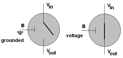
A transistor has three
connections, a base B an emitter, Vin, and a collector Vout.
The base acts as a switch: If the base is grounded,
the
emitter is not connected to the collector. If a voltage is applied to the
base,
an electrical connection is enabled between emitter and collector. Vin
is always connected to a source that might have a voltage on it or be
grounded or be disconnected, while Vout may either be
disconnected or grounded (but not have a voltage attached). The standard ground symbol
is shown at the bottom of each diagram below. A capital V is used
to mean a current voltage source. The current connection of
the output to voltage or ground is shown by a gray path.

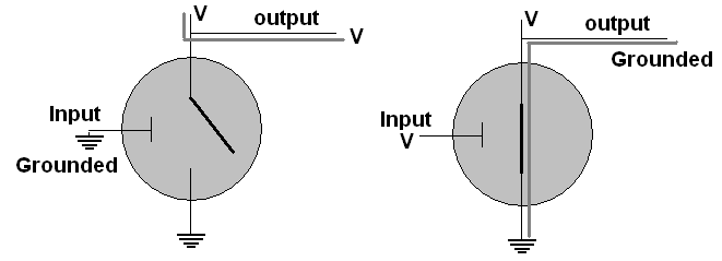
In the simplest situation, Vin
is definitely connected to a voltage source and also to an
output wire. Vout
is grounded. In this case state of the base in the
only thing
variable. If it has a voltage, the emitter circuit is
connected,
and ground at Vout is connected to Vin
which
we assumed conected to the output, so the output becomes grounded.
If the base does not have a voltage, the connection between
the
output and ground is broken, and the output is just connected to the
regular voltage source, resulting in a voltage on the output wire.
Possibilities
in the Figure
| Base | Output |
| voltage | grounded |
| grounded | voltage |
The
circuit provides out the opposite of what it gets in. If we
associate voltage with 1 and grounded with 0, we get the NOT truth
table! The NOT operation takes only a single transistor.
Possibilities in the Figure
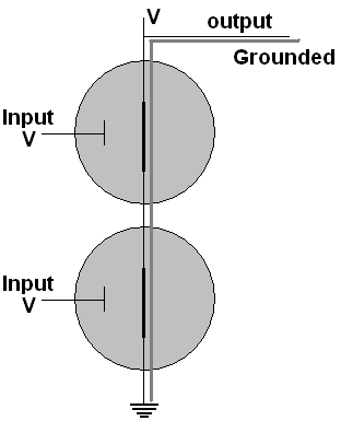
We
can connect two transistors in series as shown and use both bases as
inputs feeding one output.

Only
when both inputs have voltage, as shown, is there a connection between
ground and the output. If either input were grounded, the
connection of ground and output would broken. Hence if we
call
the inputs A and B and the output X, we get
Truth
Table for a Nand gate:
This
the truth table for NOT AND, or NAND as it is called.
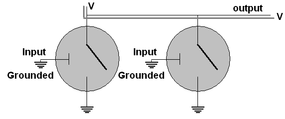
We
can also connect two transistors in parallel as shown, still using both
bases as inputs feeding one output.

The
only way to avoid a connection fbetweenthe output and ground is to
have both inputs grounded, as shown above, resulting in
voltage at
the output. If at least one input has voltage, the output
becomes
connected to ground. Hence if we call the inputs A and B
and the output X, we get
Truth Table for a Nor
gate:
This
is the truth table for NOT OR, or NOR as it is called.
To
turn the Nor into Or, a further NOT operation is
needed on the output,
requiring one more transistor. Similarly to convert Nand to
And.
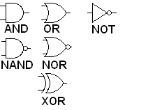
In
circuit diagrams, the details of the combinations of
transistors, voltages and
grounds needed for the different Boolean operations discussed is
hidden. The operations are given special, more simple symbols:

The
inputs are assumed to come from the wires on the left and the output
from the wire on the right. All the gates that involve "NOT"
have
a small circle where the NOT operation would take place.
For
example the Boolean expression A(B+C) corresponds to the circuit diagram

Each
input is assumed to correspond to a voltage on a labeled wire, usually
coming from the left. These wires feed gates with result
wires coming out of them. As long as each wire ends up going
to the left, each wire corresponds directly to one Boolean expression.
Following the wires, putting the symbolic result labeling
each one in turn, eventually leads us to an output. These are
sequential
circuits. Circuits with loops in them are also important, but
more complicated. They are call combinatorial
circuits.
We
will mostly work in terms of AND, OR, and NOT, because of their
familiarity, though NAND and NOR are used more in actual engineering
practice, since they require fewer transistors in a circuit.
By
putting more than two transistors in series or parallel, NAND
and NOR gates with more than two inputs can be constructed, hence
with a further transistor, multi-input AND and OR gates can be
constructed. The same AND and OR gate symbols are used in this
case, except more input wires are allowed.
Class
25
In the introduction, I mentioned
that we want to be able to convert between all these representation.
We have discussed the direct translation between Boolean
expressions and circuits, and we have shown how to convert a Boolean
expression into a truth table. The only direction missing now
is from truth table to Boolean expression.
Finding
a Boolean Expression for a truth table
A B C X Example
0 0 0 0
0 0 1 1
0 1
0 0
0 1 1 0
1 0
0 0
1 0 1 1
1 1
0 0
1 1 1 1 <- First find expression producing
this 1 and = 0 everywhere else
A
B C X
0 0 0 0
0 0 1 1
0 1
0 0
0 1 1 0
1 0
0 0
1 0 1 1 <- Find
expression producing this 1 and = 0 everywhere
else
1 1 0 0
1 1 1 1 ABC
A B C X
0 0 0 0
0 0 1 1
<- Find expression producing this 1 and = 0 everywhere
else
0 1 0 0
0 1 1 0
1 0
0 0
1 0 1 1 AB'C
1 1 0 0
1 1 1 1 ABC
A B C X
0 0 0 0
0 0 1 1
A'B'C
0 1 0 0
0 1 1 0
1 0
0 0
1 0 1 1 AB'C
1 1 0 0
1 1 1 1 ABC
Have expressions = 1 ONLY in each place X is 1
X = A'B'C + AB'C + ABC (each of the expressions OR'ed)
A circuit could certainly be made for X, but it would be
easier with a simplification. One advantage of Boolean algebra is
that it is easy to manipulate algebraically, for instance using the
rules of Boolean algebra above. I will not hold you responsible
for this, but it will shorten some answers. Focus on the second
two terms:
A'B'C + AB'C + ABC
= A'B'C + AC(B'+B) distributive rule (factoring out A and C
= A'B'C + AC(1) complement rule for OR
= A'B'C + AC identity rule
One general rule that is easy to check that was not in the earlier rules is
A + A = A, or with A replaced by AB'C
A'B'C + AB'C + ABC
= A'B'C + AB'C + AB'C + ABC adding a second ORed copy of AB'C
= (A'B'C + AB'C) + (AB'C + ABC) associating the parts we want
Just as we showed AB'C + ABC = AC, we can rework the first two terms:
A'B'C + AB'C = (A' + A)B'C
= (1)B'C
= B'C
The
general pattern that simplies is when all but one factor matches
in two terms, the nonmatching term (negated in one term and not negated
in the other) can be completely removed.
In this case, using these simplifications, the original expression
A'B'C + AB'C + ABC
= B'C + AC or use the distributive property again:
= (B'+A)C down to 3 operations from 11 in the original expression
Find a truth table for the Boolean expression that is true when all three inputs
(A, B, C) are the same (call this X initially). Then find the Boolean expression itself.
A B
C X
0 0 0 ?
0 0 1 ?
0 1
0 ?
0 1 1 ?
1 0
0 ?
1 0 1 ?
1 1
0 ?
1 1 1 ?
A
B C X
0 0 0 1
0 0 1 0
0 1
0 0
0 1 1 0
1 0
0 0
1 0 1 0
1 1
0 0
1 1 1 1
Now what?
A
B C X
0 0 0 1 <- First
find expression matching this 1 and = 0 everywhere else
0 0 1 0
0 1
0 0
0 1 1 0
1 0
0 0
1 0 1 0
1 1
0 0
1 1 1 1
A B
C X
0 0 0 1
A'B'C'
0 0 1 0
0 1
0 0
0 1 1 0
1 0
0 0
1 0 1 0
1 1
0 0
1 1 1 1
<- Then find expression matching this 1 and = 0
everywhere else
A B C X
0 0 0 1
A'B'C'
0 0 1 0
0 1
0 0
0 1 1 0
1 0
0 0
1 0 1 0
1 1
0 0
1 1 1 1
ABC
Then what?
Combine:
X = A'B'C' + ABC
Download gates files under examples
Class
25
Bring up lab 7.1, do it. Also construct a tester
for a Boolean
algebra identity (other than those done in class) for the other
distributive property or for complement or for the other DeMorgan law.
Computer circuits:
In all our logical operations, we did not see normal
arithmetic, but we want that! Since we are using two state
circuits we will do binary arithmetic. If we stick to 1 bit
additions, there are not many choices:
0 0 1 1
+0 +1 +0 +1
-- -- -- --
0 1 1 10
The
complication is the carry in the last case. It means we need to
keep track of two binary outputs, sum (the 1's bit) and carry (the
carry bit):
Truth
Table sum and carry in binary addition
| A | B | carry | sum |
| 0 | 0 | 0 | 0 |
| 0 | 1 | 0 | 1 |
| 1 | 0 | 0 | 1 |
| 1 | 1 | 1 | 0 |
It turns out you may recognize both the outputs: carry is AND and sum is XOR. The book uses AND and OR gates for XOR
A XOR B = AB' + A'B
See gates applet with examples halfAdder.dat
When
you do addition using place value with two multi-digit numbers x, y,
you actually have to add three digits together at a time in general:
a digit from each number x and y, and a possible carry from the previous place. An example as you might have written it in primary school to add 5147 and 7689:
11
5147
+7689
-----
12836
In
binary that means adding three inputs that can be 0 or 1, with a sum at
most 3, still only needing 2 bits of output. We can put two half
adders together, as in Figure 7.8, or as in example fullAdder.dat.
Once you have full adders you can chain them together as in figure 7-10 or in example 3bitAdder.dat
See Program 7.
Lab time
Class
26
Exam 3 Class 27
HW2: on paper in class next Tuesday May 2. Individual
assignment!
Be sure to do the reading assignments in the Analytical Engine for the next class: we will be having a class discussion.
Other circuits needed for a computer.
Multiplexor:
choose a data line. Input consists of a power of 2 data
lines and control lines which choose a data line to go to the one
output line. See Multiplexor.dat It shows 2 data line and 1
control line (the control line can choose between two states).
There could be 23 = 8 data lines and 3 control lines (3 control lines can choose between 23 states).
A demultiplexor does the reverse: n control lines and one data input line deliver the input value to one of 2n output data lines.
Memory:
We have only considered sequential circuits - signals flow
through and nothing is kept. We need a combinatorial circuit, one
with a loop in it, to have memory. Loops can get tricky.
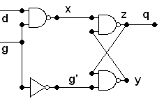
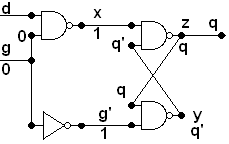
A latch can remember a value.

It
has two main direct inputs d, the data value, and g, which is 1 as we
shall see when the circuit should get the data. Note the two
lines feeding back: y, z. Also z goes to the output q.
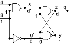
These are nand gates so x = (dg)'; z = (xy)'; y = (g'z)'
If
g is 1 and g' is 0, this simplifies to x = (d1)' = d' = 1; y = (0z)' =
(0)' = 1, so z = (d'1)' = (d')' = d, and this is passed to q:
that means the value of d is transmitted to the output, however
it changes.


If
g is 0 and g' is 1, it is more complicated and we mut take the old
value of y = q', z = q, into account. x = (0d)' = 1, and d has no further
effect. y = (1q)' = q' which then circles around to make z =
(1q')' = q, which is what it was before, so the loop maintains its old value, independent of how d is changed!


It
is not quite that simple if you look at latch.dat in the lab 7.1
applet. If you try to run it (with lower input g = 1), you can
switch the upper input d and have it behave as expected. However
if you change g to 0, you should see the circuit flash continuously:
That transition of g
from 1 to 0 is a problem. This is a timing issue. Load
latchWorks.dat. See that two extra NOT gates are inserted.
In a static logical state they cancel each other out, but they
change the timing when the
signal from g alters and splits. Now try running the applet with
any sequence of input data, and it should work. When the lower
input (g) is 1, the output changes with the upper input (d). When
g is changed to 0, the last output is remembered, no matter what you do
later to d.
This
example indicates the importance of timing. We have left out a
discussion of the regular alternating clock signal that is used to
stablize outputs.
We have illustrated the main circuits in a
computer: A more detailed schematic than in my pipGui.py is in
the Applet for lab 6.1, and if you follow the lab, you can see some
internal operations in the middle of executing instructions.
