Algorithms, Web Page 06
Some Dynamic Data Structures
Back to Amortizing.
If you download this page, note that you should also download the
subdirectory b-trees to be able to see the graphical images.
One way to do that all at once is to download 06BTree.zip.
Dynamic data structures allow lookups and change based on their
use: in hash tables and B-trees there can be additions and
deletions.
Another form of dynamic data structure in a union-find tree. This
structure has a rather specialized use, and I delay discussing it until
after we introduce a greedy graph algorithm that can use it, and give
it context.
Hashing (Book section 7.3)
I assume you saw hash tables in Comp 271. Review the three forms of hashing, for instance by reading the book section.
WARNING! Very misleading terminology in the book: What I will call chained hashing, the book call "Separate chaining" or "open hashing".
Completely different are the versions of open address hashing, which
the book also calls "closed hashing", so open is used in totally
different ways in the book. Henceforth, I will only use "open" in
connection with open address
hashing. As in the book, I distinguish the two general approaches
to open address hashing as "linear probing" or "double hashing".
For short, open linear and open double.
Average Timing
Let α be the load factor in a hash table: the ratio
of keys to
total array elements. In
chained
hashing, α is the average length of the linked
lists. In a
successful search, the desired key will be on
average about
half way down, so the will be α/2 failed comparisons followed
by 1
successful comparison, or 1 + α/2 on average.
For open address hashing, the analysis is much more difficult
and was
carried out exactly by Knuth (see the references at the end of the
chapter) in the case that there are only additions, not deletions from
the table. In this case the average number of comparisons is
Open address hashing with linear probing: 0.5 +
0.5/(1 - α)
Open address hashing with double hashing:
-(1/α)ln(1 - α)
Average Number of
Hash Table Comparisons
----------------------------------------
Load
Open Open Chained
Factor Linear
Double
0.25
1.17
1.15 1.13
0.50
1.50
1.39 1.25
0.75
2.50
1.85 1.38
0.90
5.50
2.56 1.45
0.95
10.50
3.15 1.48
0.99
50.50
4.65 1.50
1.00
----
---- 1.50
1.50
----
---- 1.75
2.00
----
---- 2.00
2.50
----
---- 2.25
This table was printed using hashAvgComp.py,
in the handouts on the web. This table is somewhat
misleading, as your homework problem E gets you to explore.
You should understand the algorithms for each of these three
versions
of hashing, and be able to show the sequence of changes to a hash table
made for any example listing the size of the array and the values of
the hash codes for each key added or removed (plus for double hashing,
second hash value -- the increment used to resolve collisions).
The book mentioned that
prime length hash tables are a good idea in case you have an imperfect
hash function. (For instance if your hash function ends up always
being even, and the hash table has and even length n, then the target
index h mod n will always be even - wasting half the hash table. The
common factor is the issue. A prime length avoids that. For double
hashing there are only n-1 places you want to look with the second hash
(since you assume a collision at the first place). You could make the
increment be the original hash value h mod (n-1), but n-1 will
alway be even if n is prime. Not good. Knuth noted, however, there are an infinite
number of double primes pairs p, p+2 (3:5, 5:7, 11:13, ...). If the
prime N is the larger of a double prime pair (2 apart), then
if h
is the hash value for a key, the index for the first try is
the
usual h mod N. For the double hash, you want an easily
calculated, apparently independent increment 1, 2, .... N-1.
An
easy an excellent choice uses the already calculated h: 1 +
h
mod (N-2). The only defect here is that it takes on one fewer
value (N-1 is impossible). I use a double hash increment
chosen
in this way for the examples below.
Hash Table Algorithm illustrations
Assume a hash table of size n = 13, to which we want
to add a number
of names as keys. The arithmetic for a sequence of names is
shown.
Hash codes given are the actual Java String hashCodes. The
index
is
Math.abs(key.hashCode()) % n. Also shown for double hashing
are
the
increments used after collisions 1+ Math.abs(key.hashCode()) %
(n-2). Note the use of absolute value. Hash results are
usually arbitrary machine integers, half or which are negative.
-13 mod 5 is -3, not a good index. The abs avoids that
problem. (You could also use an if statement and add n if the
modular result is negative.)
Key
HashCode Index Increment
----- -------- -----
--------
Phu
113485
8 10
Amy
93139
7 3
Miao
4047726
7 2
Jose
3904637
9 1
Liz
108051
8 10
Eve
98928
11 6
Xiao
4604909
10 2
Abe
92712
9 5
Consider adding just the first three names to the
hash table, in the
order given. I show three columns, one for each of the three
hashing
methods: open addressing, double hashing, and chained
hashing.
'/' is used to mean null or nil for the linked lists.
open
double chained
0
/
1
/
2
/
3
/
4
/
5
/
6
/
7 Amy Amy
-> Miao ->
Amy -> /
8 Phu Phu
-> Phu -> /
9 Miao Miao
/
10
/
11
/
12
/
Hash Example a: Add the
next three names to
the hash table in the same format. Answer
a
b. Now imagine that Liz is
removed. How would the
table look then? Answer b
c. Now add Xiao and
Abe. How would the table look
then? Answer c
Comparisons to Other Dynamic Data Structures
Hash tables have operations that all amortize to O(1). Why do
we
look at any other dynamic data storage methods? Hash tables
are
much used. They do have drawbacks of extra memory usage, bad
worst case time, and (intrinsic to hashing data up) a loss of
order information. See the following examples in Java:
//Simple Hashtable example with use of an iterator
import java.util.Hashtable;
class HashTest {
public static void main(String[] args) {
Hashtable<String,
Integer> numbers = new Hashtable<String,
Integer>(); // String key, Integer value
numbers.put("one", 1);// first
parameter is the key, second the value
numbers.put("two", 2);
numbers.put("three", 3);
numbers.put("four", 4);
numbers.put("five", 5);
for (String key : numbers.keySet())
System.out.println(key + " : " + numbers.get(key));
}
}
Run this program and note the order that the numbers are
printed out!
When the keys get hashed, their order depends on the hash codes and the
hashing algorithm used, which is implementation dependent!
Hashing Exercise
1. Same idea as the Example above (minus the
actual Java
hashCodes): Suppose the following actions are done in
order. Show the state of a hash table of size 7 for all three
versions of hashing. Assume there is no rehashing into a
larger
array -- even though the table gets rather full. The order
inside
linked lists is not important.
Action Key Index Increment
------ --- ----- ---------
Add
A 0
3
Add B
5
1
Add C
0
2
Add D
5
4
Add E
6
6
Delete D
5
4
Add
F
5 2
open double chained
0
1
2
3
4
5
6
Balanced Trees
This is a mostly self-contained section on B-trees, with some
references to see how Red-Black Trees relate. The book has a brief introduction to B-trees in 7.4, and a
treatment of the special case of 2-3 trees in 6.3.
Binary Search Trees
Search in a Binary Search Tree is O(tree depth). The depth can be
O(lg n) but it
can also be O(n) if earlier insertions and deletions in the binary tree are
done
naively. There are several variations on search trees that
keep
the depth at O(lg n): Balanced trees, AVL trees, and Red-Black
trees. Red-Black trees are a very popular
version for
trees held entirely in memory. The red-black algorithms are
hard
to
motivate directly (for me), but they are related to the much more
accessible and separately useful B-trees.
All of these approaches have trade offs, but not of space and time as
the book suggests in its chapter title, but between time to maintain
the data structure vs time to do searches, insertions, and deletions.
B-Trees
I refer to the data to be searched as data values.
The book uses keys. For the algorithm, the further data that goes
with the key is irrelevant to the algorithm, as with a hash table.
B-trees are not binary trees. They typically have
multiple data
values in each node, x1, x2,
...xk,
and in a node where there are k data values
there are k+1 child nodes. We define them in two
steps. The
first is my term for a generalization useful in the middle of
transforming B-trees. The second term is standard:
Generalized
B-tree of height h >= 0
The only generalized B-tree of height 0 is nil.
A generalized B-tree of height h > 0 has a root node which may have
zero
or more data values. This number of data values is its size;
denote it by k. Name
the data values xi, 0 < i ≤
k. The node also has
k+1 indexed subtrees T0, T1,
T2,
... Tk with the following properties:
Each Ti
is a general B-tree
of height h-1.
The values xi are sorted in nondecreasing order.
The data in non-nil subtrees is interleaved by the data in the
node: If Li and Hi
are the lowest and
highest data value in the whole subtree Ti,
Hi-1
≤ xi ≤ Li
for i = 1 to k.
An m-M tree,
or just B-tree
if m and M are known in the
present context, is a
generalized
B-tree with the additional restrictions:
m and M are integers with 2 ≤ m, and 2m-1
≤ M
If the tree is non-nil, each node except the root
satisfies m ≤ number of children ≤ M, or equivalently m-1 ≤
size ≤ M-1, and the root
node satisfies 2 ≤ number of children ≤ M, or equivalently 1 ≤
size < M.
In some definitions M is required to equal 2m-1. If the value
of
M is small, all the possible number of children may be listed in the
name, as in 2,3,4 tree
rather
than 2-4 tree.

The recursive definition gives an equal depth to all child subtrees. Hence all leaf nodes are at the exact same depth.
Note that a B-tree may be efficiently searched. If a desired
target is not in the root node, there is just one subtree that need to
be searched recursively to find it, similar to a binary search tree.
We wish to discuss algorithms for inserting elements into and deleting from
B-trees. At intermediate points, generalized B-trees may be
created. There are two basic transformations (plus their
inverses) on generalized B-trees that need to be considered:
promote
and split
and its inverse demote
and join.
shift
right and
its inverse shift left


In the shifts, note that subtree between the two moved data nodes
switches between the two subtrees (to stay between the two moved data
nodes).
For generalized B-trees, when the red data exists, these
transformations
can always be made.
Insertion and Deletion in a B-tree for a set
Repeated elements may be allowed when adding to a
B-tree.
We will consider the case when the B-tree represents a set of data
values, so no repetitions are ever stored. Both of these algorithms
modify the B-tree on which they act, and may end up with a different
object as the root. They also return true if the B-tree was
changed, and false if it was not.
boolean
insert(target)
- If the tree is empty, make the tree have one node
with just the
target as data,
and return true.
- Otherwise, keep track of the subtree that
the target might be found in. If
it is not found in the root via binary search, continue in the one
subtree that
it could be found, until
- It is
found, return false
- Else a node at
the bottom of the tree is reached and the target
is not in the node.
The rest of the procedure allows one node to have size M,
and
if one does, as the tree is transformed that node moves up the tree,
possibly going all the way to the root. - Initially add the
target
to the bottom node, inserting it in order.
- While the node with the
insertion or promotion is not the root
- If the
node is still of size less than M, return true.
- Else
the size of the node is M. Since M >= 2m-1,
promote
the middle element and split the node in two, both of which will have
legal size, at least (2m-1 - 1)/2 = m-1. To make each choice
unique when demonstrating the algorithm, you can insist that
if the two parts are of
unequal size, the left sibling node ends up one smaller than the right
sibling node. The loop now focuses on the node with the promotion.
- If this
point is reached, the root has size M.
Create a node with
no data above the root, and promote the old root's middle item into
it. Then this new root has size 1, which is always legal for
the
root, and the new
root's two children will have size at least m-1 as in 4b, so the the
tree is an
m-M tree with height one more than previously. Return true.
Example: Starting with the 2-4 tree of height 3
displayed above,
suppose 34 is inserted. The sequence of generalized B-trees
created is shown, with the node which might be keeping the tree from
being a 2-4 tree
shown in yellow, with red arrows showing what the next promotion will
be:


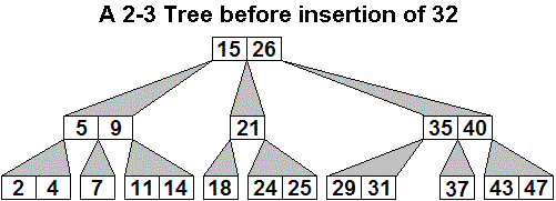
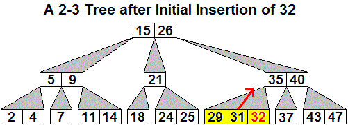
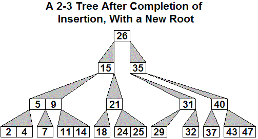
Here is an initial 2-3 tree, then the generalized tree with
32
inserted, and then the final 2-3 tree after three promotions, including
the last which creates a new root.


The only way the height of the tree increases is when step 5 is reached
and there is a promotion out of the original root node, as in the last example. Extending at the
top means all the leaf nodes still have an equal depth, but now one
more than it was before.
boolean
delete(target)
- Search for the target. If it is not
found, return false.
- If the target is found,
there are two cases
- The target
was found at the bottom level or
- The
target was found at a higher level. In this case
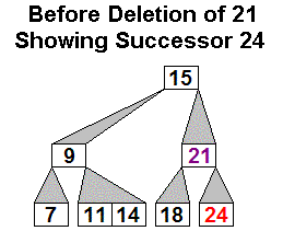
- Traverse
the tree down to find the successor of the target
at
the bottom of the tree by going to the subtree to the right of the
target, and following the tree down its leftmost subtree to the
leftmost element of a leaf node.
- Overwrite
the element to be deleted with this successor
- Switch
so the copy of the successor at the bottom of the
tree
is the element to be removed
At this point the element to be removed is at the bottom
level. As in the insertion algorithm, in intermediate steps
hereafter one node may have an illegal number of elements -- in this
case one too small, m-2. Levels will be resolved one at a
time,
possibly making a change to the parent level that will make it too
small, possibly extending all the way up to the root, leaving it too
small (size 0): - Remove the element to be deleted at the
bottom
level.
- While the node
with an element removed or demoted is not the
root with size < m-1: fix the possibly small size node:
- If its
node still has size >= m-1, return true.
At this point the node is too small, of size m-2. Since the
node
is not the root, it must have an adjacent sibling.
- If an adjacent sibling has size more than m-1,
use the left or right shift transformation to reduce the size of the
adjacent sibling by one (and it will still have size >= m-1) and
increase the size of the deficient node, making it have size m-1, so
this
node is fixed without making a deficiency elsewhere. Return
true. To make each choice unique when demonstrating
the algorithm, you can insist on shifting out of the larger
sibling node or out of the right sibling if both are of the same size.
- Else (an adjacent sibling has
size m-1): perform the
demote
and join transformation, joining the deficient node (with size m-2) and
the adjacent sibling (of size m-1), adding the demoted
element,
so
the joined node has size m-2 + m-1 + 1 = 2m-2 < M, so this node
has
a
legal size, but now the parent is the possibly small node.
To make each choice unique when demonstrating the
algorithm, you can
insist on joining with the right sibling if there are two adjacent
siblings of size m-1.
- If this point is reached, the possibly small
node is
the root. It only needs to be fixed if it has no
elements. In that case the node has only one subtree, and the
empty root can be removed and let its subtree be the new
root.
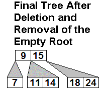
Return true.
Deletion Example 1:


Example 2:


CAUTION: Deletion example
2 carefully shows the intermediate versions where a node N has shrunk
to 0 elements (shown as yellow lines). It is easy to forget that
node, and just omit N so N's parent becomes directly connected to N's
one child. This is wrong.
A node cannot change depth relative to other nodes, and all leaves are
always at the same depth in a B-tree. That property is broken by
mistakenly connecting N's parent to N's child, originally two levels
below. The only way levels change is when an empty root
node is removed, and then the depth of everything changes Lower
level empty nodes are only resolved by shift left or right or by a
demote and join: These changes reconfigure nodes but do not change the
number of levels.
Time bounds
Search at worst traverses to the bottom of the tree. Insert
at
worst traverses to the bottom and then fixes ancestors on the way back
up. Delete at worst searches
and finds
the successor all the way to the bottom of the tree and then fixes
ancestors on the way back up. All traverse the depth of the
tree
at most twice. All are O(the tree's height), assuming we
consider
M to be O(1).
Depth bounds
Since all leaves are at the same depth and all nodes but the root
branch at between m and M times, the number of data values at the
lowest level, b can be bounded (M-1)Mh-1
>=
b >= (m-1)(m)h-2, if the depth
h >1.
Taking logs we see log b is Θ(h), and hence h is
Θ(log b). Since
the lower level has more than half the elements, b is Θ(n),
and the
depth h is Θ(log n). (The proof or the relation
between b and n
is an exercise below.)
Hence all of the operations search, insert, delete are O(log
n).
Back to binary trees
B-trees are useful with various m-M pairs. Enormous databases
which have to be mostly stored in disk files tend to have a large m and
M so that one node uses array storage corresponding to a disk
sector. Search within the array data is via binary search.
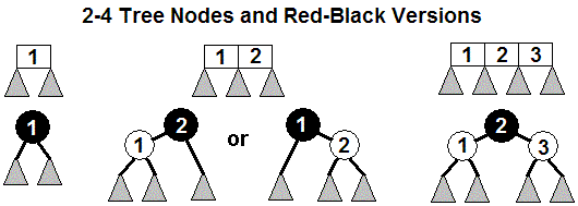
Binary trees do have a certain simplicity. A 2-4
tree can be
implemented as a binary tree: If there is a single data value
and
two subtrees, they can be stored via a single binary tree
node.
If the 2-4 node size is two or three, it can be modeled with 2
or
three binary tree nodes. The one complication is that in a
traversal down from the top of the tree, some nodes indicate the start
of a 2-4 tree node, but there are extra binary tree
nodes corresponding
to a 2-4 node with 2 or three data values, and it is not clear where a
B-tree 2-4 node starts and ends. To keep the correspondence with
2-4 trees, one extra
bit of information is needed for each binary node, typically indicated
as a choice between red or black coloring, where black indicates the
start of a new level of the 2-4 tree, which may be connected to one or
two red nodes that would be part of the same 2-4 node. The
figures below indicate the correspondences for the different sizes of
2-4 node. In the pictures in this page, red is replaced by
white.

Full tree example

A 2-4 tree modeled in this way is a red-black tree.
The book has a
rather different looking definition! Comparing terms, we see
the
black height of a red black tree is the corresponding height of the
B-tree. The red-black trees are generally drawn with all the
nodes modeling one B-tree node at the same level, reinforcing the
correspondence with 2-4 trees.
Since a red-black tree is actually a binary search tree,
searching is
the same as for any binary search tree (the color information is not
needed). Algorithms for insertion and deletion could be
worked
out as direct translations of the B-tree algorithms given above, and
they would be still be O(log n). In fact, the algorithms can
be
made somewhat more efficient (though not always easier to follow!) by
taking
further advantage of the particular red-black binary tree
implementation.
I am skipping the
lengthy
red-black tree algorithms. We have outlined how they are
binary
trees with a color attribute that allow searches, insertions, and
deletions in O(log n). I do
hold you
responsible for the B-tree algorithms, and the relationship between 2-4
trees and red black trees, specifically how you can convert
between
a 2-4 tree and a red black tree, in either direction.
I'm not sure why this section is under space-time tradeoffs in the text. There is a
space-time tradeoff in one common use case: where the data does
not fit in memory. In that case slow disk reads are decreased by having
each node bigger, but this takes up more space in memory.
Exercises.

- Show the result of this insertion algorithm after
insertion into
the 2-3 tree above. To save time you only need to show the
nodes
that change and child links of those nodes, with "..." under children
whose subtree does
not change:
- Insert 193
- Insert 52
- Show the
result of this deletion algorithm starting from the
original 2-3 tree above. Again, you may just show a partial
tree.
- Delete 80
- Delete 250
- The delete
algorithm needed to include a case which does a right
or
left shift. Right and left shifts are not necessary, but
possibly helpful in the
insert
algorithm. Modify the insertion algorithm to possibly
terminate
the
loop that goes through ancestors by doing a shift. You do not
need to totally rewrite the algorithm, but clearly refer to how the
parts you write out fit into the parts that you are keeping from the
original algorithm.
- Prove
my claim that more than half the elements of a non-nil
B-tree are in the lowest level, for any legal values of m and M.
This is a challenge for most students. It depends
strongly
on the fact that nodes not at maximal depth have one more subtree than
data elements.
- Draw the B-tree corresponding to the red-black tree
below.
I did not use graphics; The Black nodes have B before the
numeric data. The dots are just spacers, so if you view the
diagram in a fixed width font it looks right..
.............B30
........../........\
.......B15.........B50
...../....\......./....\
..10.....B18....40......75
../ \.........../ \...../ \
B5..B14......B35 B42..B60 B90
..\......................./ \
...7.....................80 95
On to basic graph traversals.
Hash table example solutions:
Answer a.
open----- double chain
0
/
1
/
2
/
3
/
4
/
5
Liz
/
6
/
7 Amy Amy
-> Miao ->
Amy -> /
8 Phu Phu
-> Liz ->
Phu -> /
9 Miao Miao
-> Jose -> /
10 Jose Jose
/
11 Liz Eve
1 -> Eve -> /
12 Eve
/
Answer
b.
open----- double chain
0
/
1
/
2
/
3
/
4
/
5
vacated
/
6
/
7 Amy Amy
-> Miao ->
Amy -> /
8 Phu Phu
-> Phu -> /
9 Miao Miao
-> Jose -> /
10 Jose Jose
/
11 vacated Eve
-> Eve -> /
12 Eve
/
You might have used some other notation, but the
point is that the
vacated
spaces must not appear exactly the same as the spaces that were never
occupied!
Imagine you are searching for Eve now. In the open
addressing,
you would not want to stop at empty location 11 and decide that Eve was
not present.
Answer
c.
open----- double chain
0 Abe
/
1
Abe
/
2
/
3
/
4
/
5
vacated
/
6
/
7 Amy Amy
-> Miao ->
Amy -> /
8 Phu Phu
-> Phu -> /
9 Miao Miao
-> Abe -> Jose
-> /
10 Jose Jose
-> Xiao -> /
11 Xiao Eve
-> Eve -> /
12 Eve Xiao
/
On to basic graph traversals.


