Graph Traversal

Back to Some Dynamic Data Structures

Graphs – Depth and Breadth first Search (Text 3.5)

Note: Text section 3.5 gives two numbers as subscripts to each vertex in the illustration at the top of p. 123.  Ignore them.  There are two issues with these numbers: 

• The version of DFS at the bottom of p. 123 only sets the first number.  The second number is not addressed at all explicitly.
• This numbering system is DIFFERENT and less useful than the active interval I develop below and is also used in DasGupta. Use only my/DasGupta's version!
  

Big and ongoing topic! Emphases:  understand basic definitions, matrix and adjacency representation of graphs, breadth first and depth first search, and some simple algorithms based on them and some that use the more complicated classifications of edges.  In general understand the idea of adding to DFS and BFS to obtain various objectives. Understand logical arguments made with graph ideas and make simple logical arguments.

Make data structures concrete with example.

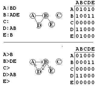
Below are edge list and adjacency matrix interpretations for an undirected and a directed graph.  (These representations go back to section 1.4 in the text.)

Like the book, I will follow the practice of labeling vertices with capital letters, avoiding any confusion with various uses of numbers that will later be associated with graphs.  In efficient implementations the vertices are just associated with numeric indices.

Download and see handouts for depth-first search:

• DFS.py, most basic.  Python reading questions?  Note most of the code is to display things conveniently, used in other programs, too, but NOT required for the course! 
  
• Switch rapidly to DFSIndent.py, showing off stack order more clearly,
  
• then DFSEdgeClassify.py for edge classification in undirected graphs (where only tree and back edges are possible), 
  

You should be able to demo these versions by hand, without  executing, for small graphs. 

Note on the programming style:  This procedural versions of dfssweep and dfs need to be changed for each different application, though most of the code is the same.  Later I develop an OOP version, which avoids this via subclassing.
 
An alternate search approach is breadth-first search BFS.py.  We can show its closeness  to DFS with a non recursive explicit stack DFS implementation DFSStack.py.  If you want to separate distances, you can use two queues, BSFDist.py.

Many things can be done by inserting code into the basic DFS, and to a lesser extent, BFS.

I will generally use V as the vertices of a graph and E as the edges and |V| and |E| as their sizes.  All of the algorithms have order |E| + |V|: the main body of dfs or bfs is called once for each vertex, and the inner loops are executed once for each edge.  All the elaborations add only an extra O(1) each time they are executed in the basic flow. 

Given that the number of edges can vary up to Θ(|E|²), the order may be from Θ(|E|), with a sparse collection of edges, to Θ(|E|²), with a dense set of edges.

Assuming  fixed size descriptors for each piece of the data, the total size of the data has the same order as the time of execution, and the algorithm time order is said to be linear (in the size of the data). 

How could you label connected components to an undirected graph? Done in 163? My solution in Python: DFSComp.py. I use the index of the first element found for a component as the component index.  (The definitions and algorithms need to be adjusted for directed graphs - discussed later.)

Digraphs and DAG's (4.2)

With directed edges the classifications are more complex.

Edge classifications:

Tree edge:  to previously undiscovered node
Back edge:  to ancestor
Forward or descendant edge:  to descendant previously discovered
Cross edge:  no ancestor/descendant relationship

Dasgupta, Section 3.3 p98 (page 9 of Chapter 3) has a nice digram and introduction (better than our text).  Try an example, label edges.

How do mechanically?  digraphEdgeClassify.py illustrates some approaches.

Note the order of the start of visiting (None indicates still not visited)
Note the order of finishing visiting (not yet finished None)

If u is first visited after a vertex v is first visited but before  v is finished, u is a descendant of v. (Everything on the stack after v is a descendant.)

The edge to such a u when u is first discovered is a tree edge.
The edge to such a u, but after u first discovered, is still to a descendant, but now the edge is forward
Conversely an edge from u to ancestor v would be back.

The remaining case is when there is no ancestor-descendant relationship. This is a cross edge. This occurs when dfs is working on v, and looks to a neighbor u that is already finished.

Why can't forward and cross edges occur in an undirected graph?

You cannot finish with a vertex in an undirected graph when a vertex directly connecting to it is still unvisited.  In a directed graph there can be a connection to a finished vertex - as long as the reverse edge is missing.

DAG: Directed Acyclic Graph

In an operating system, at the most abstract level, how do you get deadlock?

You have a collection of processes waiting for (dependent on) other processes.  This gives a dependency graph. 

A convention needs to be maintained with a dependency graph.  You can either have the arrows go with time, from what must come first to what must follow later (as the book does it) OR you can have a task point to the things that must be done first, reversing all the arrows in the text.  This latter approach is actually more useful for further algorithms, making it easier to check on all prerequisites being completed, so I will use it:

task  -->  prerequisite task,  
or, since we usually diagram time from left to right:    prerequisite task   <-- task

With either convention, in deadlock there is a cycle in the dependencies.  If you expect to finish a collection of tasks with dependencies, there can be no cyclic dependency!  A workable dependency graph is a directed acyclic graph (DAG).

Topological Order:  In graph with n vertices, assign topological number t(v) = 1..n to the vertices in a way that if vw is any edge, t(v) < t(w).
Reverse topological order, r(v): backwards from above: if vw is an edge, r(v) > r(w).

Theorem: The sequence of ending times end[v] in a DFS satisfy end[v] > end[w] for edges vw.    

Proof: Need to show for any edge vw, end[v] > end[w]. Look at the four edge types:

• Back edges imply a cycle - so excluded.
• Forward, tree edges: w is a descendant of v, and hence by the LIFO sequence of the stack, the ending time for w is before v.
• Cross edge: w is already completed when the edge from v is checked.

Critical Paths (important, but not in text)

Critical paths are applications for DAG's and reverse topological order:

The last application of reverse topological order was for a sequence with a single processor or actor.  In parallel processes, (human or machine), tasks that do not depend on each other can be done at the same time. The chain of dependencies that takes the longest time determines the minimum time to completion. This longest time chain of dependencies is a critical path. 

Original DAG:

Each task is associated with a time for completion.  Also we want one final node (the DONE node, with 0 duration) depending on each originally terminal node:

With dependencies marked in this order the direction of time and the direction of the graph are backwards.  I will use start and end to refer to time, and use the digraph jargon source (for a vertex with no arrows to it) and sink (for a vertex with no arrows from it).
 
The table below gives dependencies and times required for each action.

The tasks with no dependencies are then sinks.  This example illustrates that there can be several sinks (actions with no dependencies).

For the critical path time calculation the the earliest finishing time for a task (EFT) = maximum of the EFTs for its dependencies + duration of the task.  WorstDep is the dependency with the worst (largest) EFT.

For simplicity the alphabetical order of tasks is already a reverse topological order. This means the table below can be filled in sequentially from top to bottom.

If each vertex is associated with its Earliest Starting Time (EST), then the path between a vertex and a dependency adds the duration for the dependency.  The edges to the DONE node then allows the duration of the otherwise terminal nodes to be encoded. 

If rTop is a list of the vertices in reverse topological order, then the maximal path weight and the path itself are easy to calculate. We assume we start with the vertex duration data in an array, and we need extra arrays EFT and also worstDep, if we want to recover the longest path itself.

for each vertex v in rTop:
    est = 0
    worstDep[v] = None
    for w in the neighbors of v: 
        if EFT[w] > est:
            worstDep[v] = w
            est = EFT[w]
    EFT[v] = duration[v] + est

Then the EFT for the Done vertex is the overall earliest finishing time.   Without the marked Done vertex,  there must also be a check for the vertex with the worse EFT.
Full code with testing in critPathTopo.py.  By the same logic as for the DFS and BFS, this algorithm is linear in the data size.

So the minimum duration is 18, and critical path is obtained by reversing the path from Done given by the WorstDep column.  J, F, B.  Reversed is the order of the critical parts to complete (forward in time) B, F, J.

We will come back to this topic later, but for now note that DAGs and topological order are central to dynamic programming.

Weighted graphs are a standard kind that we will discuss more later, but they weight the edges, not the vertices. We can make a weighted graph by making each edge vw get the weight or time needed to complete w. With task durations and Done vertex, and this shift, we get a weighted graph:

Showing critical paths to each vertex with the weighted edges:

You could make a weighted graph model with the vertex duration consistently either on edges to the vertex or from.  The addition of the Done vertex makes the approach I took, with the weight on edges to the dependency, more convenient.  You would have to add further edges from the sources to a Start vertex to put the weights on the opposite side.

The analog of connectedness in a digraph, and its ramifications are not discussed in our text.  There is a good discussion in Section 3.4 of DasGupta, page 101, or about the 11th page of the chapter, through the end on page 105.  You are responsible for the concepts of strongly connected components and the DAG meta-graph underling and digraph.  I have an alternate object-oriented approach to graphs in graph.py, that includes code for meta-graph algorithms DasGupta describes.  It uses other files drawgraph.py to produce diagrams that are very nice for visualizing things and graphics.py for an underlying simplistic graphics engine that I use in Comp 150, and, while waiting for you to do equivalent homework, reversegraph.cpython-36.pyc (version specific; rename to reversegraph.pyc or place the original in sub folder __pycache__). You are in no way responsible for all the math and contortions I go through in drawgraph.py to get a general algorithm for a workable image.

The module graph.py is worth discussion before getting to the parts for meta-graphs.  We will be using this module later when discussing weighted graphs.  It includes a simple Edge class which includes the edge's numerical weight. 

I save a coding step by identifying all vertices purely by name  rather than going back and forth between vertex labels and vertex indices as I do in DFS.py.  Admittedly the version with indices, which involves a basic list or array data structure, is somewhat more efficient in time than my representation which uses basically the same notation, but is dictionary based. 

The neighbor lists are modified to be lists of edges to neighbors, so the weights are included.  Rather than my kludgy list structure for a graph used before in DFS.py, vertices and edges are instance variables, and g.edges[v] is the list of edges with starting vertex v in the graph g. 

I also take an object-oriented approach to modifications of depth-first search.  In the earlier programs like DFSComp.py, I copied and then modified the code for DFSSweep and dfs.  This was not a big deal, since the code is so short.  As an alternative I use a consistent dfs_sweep and dfs that have hooks allowing all the elaborations.  All the details of the elaborations are stored a subclass of DFSHelper.  This is not any shorter generally, but it groups the elaborations together, which has some conceptual appeal. One extra piece of data I pass in dfs is the edge from the parent, which is needed sometimes (like checking if an undirected graph is cyclic). Algorithms for component finding (numberConnectedComponents), active intervals (visitOrder), and topological order (topoOrder), are included following the the same underlying ideas as DFSComp, DFSActiveInterval.py, and topoordersure.py but formatted rather differently with the OO approach.

4.4  Decrease by a constant factor

This is a special case of divide and conquer, where there is only one subcase needed, rather than 2 or more typically in divide and conquer, as with mergesort or quicksort.  We covered binary search.  I will not cover the other examples in the book. An interesting example is the Majority Problem, part b, listed as an exercise in the Divide and Conquer notes.

Next: Greedy algorithms