Algorithms, Web page 8
Greedy Algorithms, Graph and Others (Text Ch 9)
Back to Graph Traversals
Overview
A greedy algorithm is one that makes a local decision of what is
cheapest or best, without looking at whole solutions. Generally
this does not provide an optimal solution. Sometimes it does.
Guessing a greedy algorithm is often fairly easy, while showing it solves the overall problem is likely to be harder.
We first look at several graph problems where a greedy approach
can be
proved to give a globally best solution. It turns out the several
basic data structures support these graph algorithms, heaps, minheaps
with reduce key, and union-find dynamics sets. They are discussed in
more detail, too.
Spanning Tree (Applies only to undirected graphs)
In
a connected undirected graph G, a tree subgraph T that connects all vertices
is a spanning tree. In
a disconnected graph, a spanning tree is a
subgraph composed of a spanning tree in each component of G.
Minimum Spanning Tree (MST)
Given an undirected graph G(V, E) with weighted edges, a spanning tree of
minimum total weight is a minimum
spanning tree, MST.
We will look at two quite different algorithms with different
advantages and drawbacks. First, Prim's algorithm which builds
up a larger and larger connected graph:
Prim's MST algorithm for graph G
Let V be the vertices of G.
Start with an arbitrary vertex s in V.
Maintain three disjoint sets (or three classifications for vertices):
- T: the vertices in the currently connected subgraph,
initially empty
- F:
fringe (adjacent to the current tree) initially s. For each
vertex w in the fringe remember the lowest weight edge from the tree T
to w. Initially set s to have weight 0.
- U: unseen vertices, initially all but s
Also maintain a mapping, p, from each vertex to its parent in the tree,
initially all null.
while F is not empty:
select and remove a vertex v from F with minimum weight
add v to T
for each neighbor w of v:
if w is in U:
take w from U and add it to F with the weight of the edge vw
p(w) = v
else if w is in F:
if the weight of the current edge from T to w is higher than the weight
of vw:
identify fringe vertex w with the weight of edge vw
p(w) = v
When the algorithm is over, all vertices with paths from s are in
T, and p maps all these vertices other than s to their parent in the
tree T. Do an example.
See prim_mst.py
where you can execute the algorithm. Before considering the
implementation in detail, note that selecting the fringe element with
minimal weight suggests storage in a priority queue. One
implementation of a priority queue is a heap. A basic heap
implementation is in heap.py.
That, however is not efficient in this situation. Not only are elements
added and removed from the priority queue(basic operations), there is
also the need to decrease the weight of an element already in the
priority queue when a better edge from the tree to a fringe element is
found. A shortening of a "priority queue where you can decrease
the value
associated with a key" is a "priority
queue with a decrease key
operation".
Without specializing to a particular priority queue implementation yet,
the time for a graph with n vertices and m edges, assuming m >
n, is
O(n*insertItem + n*(popitem) + m(decreaseKey + getWeight))
In a basic heap there is not a way to find a specific current element,
other than a linear time search. In some cases the number of times that
a decrease key operation must be performed is Θ(|E|2), so
using a linear search could lead to a Θ(|E|3)
algorithm overall. An improvement over a basic heap in this
situation, is a heap that can do a decrease key operation in O(log |E|)
time. See heapdecreasekey.py.
The heap must keep track of both each vertex and the weight of the edge
to it, while the normal heap would just allow the smallest weight
element to be accessed. The extra structure comes with a mapping
maintained between a vertex (the key) and its position in the
heap. So you must be able to find
the entry for fringe vertex v, decrease its weight, and modify the heap
with the decreased value (bubble up the element). In heapdecreasekey.py
my notation for the lookup for
weight of vertex v in priority queue pq is pq[v]. The same
notation is used to insert a new element: pq[v] = wt, and for decrease
key : pq[v] = lowerWeight. When popping the minimum from
the heap, you recover both the vertex and the weight: (v, wt) =
pq.popitem(). Now weight lookup is O(1), thanks to the explicit
mapping, and decreaseKey causes an O(log n) bubble-up to the proper
place in the heap.
Time analysis: In this case the general expression from
above
O(n*insertItem + n*(popitem) + m(decreaseKey + getWeight))
becomes, with the elaborated heap,
O(n*lg n + n*(log n) + m(log n + 1)) = O((n + m) log n)
There are other more complicated priority queue approaches where
decrease key is O(1). The text has references. We will not
pursue them in this course.
To prove the correctness of Prim's algorithm we need a theorem, that we will also use again in the future (not in book, but is in DasGupta as the Cut Property!):
MST Cut Theorem
Suppose edges X are part of a minimum spanning tree of G = (V, E
). Pick any subset of vertices S such that X does not cross
between
S and V − S, and let e be the lightest weight edge across this partition. Then X ∪ {e} is
part of some MST.
Proof: Suppose G, X, S are as above, and T is
an MST of G that contains X, and vw is a minimum weight edge
between V-S and S.
If T also contains vw, we are done, so suppose vw is not in T.
If we add vw to T, a cycle is created with the path P in the tree
from v to w, plus the edge vw. Removing an edge from this cycle
recreates a spanning tree. Choose the edge to remove as
follows:
Since one edge of the cycle crosses between S and V-S, another edge,
v'w' must cross back Let T' = T + vw - v'w', another
spanning tree. Since vw is a minimum weight edge from V-S
to S, and v'w' is another W(vw) ≤ W(v'w') and hence W(T') ≤
W(T), but T is an MST so W(T') = W(T), and T' is also an MST.
Theorem: Prim's algorithm
produces an MST.
Proof
by induction on the number of steps so far, that the tree so
far is a
part of an MST, and hence the final step is an MST for G.
Basis: Initially no edges, certainly a subset of any MST.
Induction
step: Let T be the tree constructed by Prim's algorithm at some
step before the final one, and let vw be the next edge added, with v in
T and w not in T. Use the Cut Theorem with T = X, and S the
vertices in T, so v is in s and w is in V-S. Then since vw has
minimal weight, T+vw must be part of an MST.
In proving things about MST's the construction in the MST Cut Theorem
is standard: adding and edge, causing a cycle, and removing an
edge somewhere else in the cycle. Be sure you follow the argument.
We will return to MST's and Kruskal's algorithm, but first an
algoithm for a different problem, but with a solution almost exactly
like for Prim:
Dijkstra's
shortest path algorithm
We are looking for the
shortest path (thinking of weights as distances ) from a specified
vertex s to other vertices v, dist(v). Although the problem is
quite different than the minimum spanning tree problem, the solution
algorithm is almost the same as
Prim's MST algorithm:
The only change is that instead of priority of a candidate being given
just by edge weight vw for Prim,
it is dist(v) + the edge weight for vw for Dijkstra. In dijkstra.py the few lines with
changes are marked.
Beside examples in the text, there is an example in picture from DasGupta, Section
4.4 of DasGupta,
page 110, or about the 5th page of the chapter. See either of
these for a proof that Dijkstra's algorithm works. Be sure to
note where the nonnegative edge weight comes in.
Essentially the same analysis as Prim for time, O((n+m)log n).
Kruskal's algorithm:
Maintain a set of edges F (for forest) so far, initially empty
and the set of edges R remaining, initially all of E
while R is not empty:
Remove lightest edge vw from R
if vw does not make a cycle in F
add vw to F
return F
Proof it works - easy from MST Cut Theorem, pictured well in DasGupta
Time:
getting lightest edges takes time O(m lg m) in worst case. The
checking for components is trickier. We have already done this
efficiently in the static case, but repeating that is not efficient in
the dynamic case. There is a data structure and union-find algorithm that is
better. See pictures in our text or Ch
5 of Das Gupta. See kruskal.py,
which uses unionfind.py.
So back to the time: with the efficient version of union-find and
a maximum of 2m
finds, n-1 unions, making a union-find program of length 2m+n-1.
If we assume the usual case that m >= n (or we include some isolated vertices with no edges), this contributes O(m lg*
m), so sorting edges is the main contribution O(m lg m).
Compare
Prim: With the algorithms indicated, both Prim and Kruskal have
the same order. Depending on the specific situation, either could
be faster in practice. With fancier algorithms Prim could be
faster. If for some reason you have the edge weights already
sorted, Kruskal ends up faster.
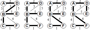
It is useful to understand the situation when there are multiple MST's
for one graph:
MST Edge Swapping Theorem (not in book!)
Let
G be a weighted graph. If S and T are
MST's for G, with k elements of S not in T, then there is a sequence of
MST's T = T0, T1, T2, ... Tk
= S, where the transition from one MST to the next involves only the
removal of one edge of T and adding of another from S of the same
weight.
Example progression:
Proof: This follows immediately by induction from the
following. Basically if you have two MST's that are k edges
apart, then you can find an MST that is one edge from one of the MST's
and k-1 edges from the other:
Lemma for the MST Swapping
Theorem:
If
S and T and G are as in the MST Edge Swapping Theorem, and there are k
edges in S that are not in T, with k > 0, then there is an MST
T' for G that is either formed from S by removing an edge of
S that is not in T and adding an edge from T that is not in S, or is
formed from T by removing an edge of T that is not in S and adding an
edge from S that is not in T.
Proof of Lemma: Homework exercise
If
you want to go up one level of abstraction, you could restate the
theorem in
terms of a graph SG, whose vertices are MST's of G and whose
edges
connect MST's differing by only the addition and deletion of one edge
in G. The theorem then says that SG is connected, and the distance from any one to another is the number of edges in one that are not in the other.
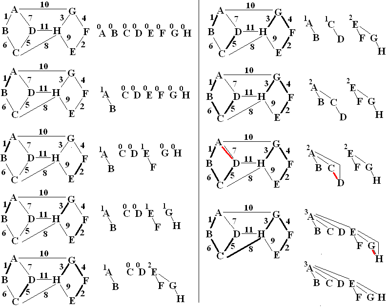
Union Find for Kruskal, Step by Step
The word rank or weight rather than depth
in used purposefully in the discussion of in-trees: Remember that
the efficient union-find gets part of its efficiency from
compression-find only traversing up from the the specified starting node up to the root, not
looking through the whole in-tree somehow. Though one path upward
may compress, you cannot assume that the compression of one path
reduces the depth, without having a full check of the in-tree.
The maximum depth (looking at the whole in-tree) may decrease, but there is no computational time given to determining that. The rank is a simple-to-keep upper bound on the actual depth. The only
way rank changes is through the simple calculation when a union of two
trees of the same rank is done, increasing the rank by 1. Rank
never decreases, so after some compression the rank may be larger than
the depth.
Assume that when there is a union of two trees with the same rank, that
the first root alphabetically stays as root. The Kruskal sequence
with the graph is at the left. The union-find data structure with
weighted union and compression find is on the right. Read down
the column first. There is one error: The
bottom of the left column's graph should not be the same as the top of
the right column. Edge CD should not yet be chosen (not thick) at
the bottom of the left column. Red is used to show a graph edge
considered, but not used (makes a cycle). Red in the in-trees is
used to indicate a removed pointer during compression. You should see
a new link added to replace it. See where compression is done and
a new edge is accepted and where compression is done even when the proposed edge is not used, since compression find is done before the final check for a cycle.
Huffman - follow our text or Ch
5 of Das Gupta pages 12..16 of the chapter.
An important characteristic of any Huffman encoding is that no bit
string used to represent a character is the prefix of any other bit
string used to represent a character.
Hypothetical Code:
A: 01
B: 011
C: 110
D: 10
How do you decode
0 1 1 1 0
0 1
1 1 0
vs
0 1 1
1 0
You avoid this problem by keeping data only at leaves.
Another clear optimization: So you do not waste nodes, there is
no need going through a node with just one
child. This means the tree structure is a 2-tree with all nodes having 0 or 2 children, never 1. (DasGupta calls this a full
tree) for a start at efficient, unambiguous decoding. There are still a lot of 2-trees.
Two ways of looking at counts are important in forming an optimal 2-tree:
1. Sum of all path lengths to leaves, with frequencies. This show
the two with the smallest frequencies should go at the bottom.
2. Also label so all interior nodes except the root with a
frequency which is the sum of their children. Each number shows
the number of paths that follow the leg from the node's parent to
itself. The sum of all path lengths with frequency is the sum of
the frequency of use of every edge, which is the sum of the values at
each node. This allows the easy
reduction to a smaller problem, replacing branch with two smallest,
just with the parent node.
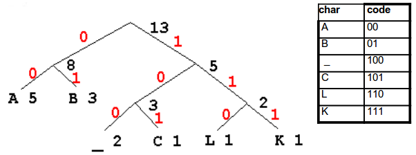
Consider “BAA BAA BLACK”
Character frequencies:
A 5
B 3
_ 2 (use _ as a shorthand for blank)
C 1
L 1
K 1
build tree, code, encode. There are multiple choices when there is not a unique smallest pair.
Python code for this is in huff.py, which uses previously discussed heap.py and a new module simpletable.py.
Class practice:
See another greedy problem: Das Gupta 5.3 Horn formulas.
Important for Prolog programming language implementation. The
claim is there is a linear algorithm in size of input to solve Horn
formulas. In DasGupta's pseudo code, the while clause could be
restated: "while there is an implication with true hypothesis and false
conclusion, change the variable in the conclusion to true". Class: work out such an O(n) algorithm. This requires carefully consideration of th data structures used.
More creative problems from earlier sections:
1. The diameter of a graph is the max of the distance
between any two
points. In particular it makes sense for a tree. Find an
O(n) algorithm for a tree (general unrooted tree, and not binary
tree). May assume all edge weights 1 for simplicity (does not
change the algorithm idea).
2. Given n professional wrestlers, with r rivalries specified between pairs. Find an
O(n+r) algorithm succeeding or
acknowledging impossibility of declaring a partition into good guys and bad guys, and have
all rivalries between a good guy and a bad guy.
3. Create an O(n) algorithm and
explain
why the algorithm has that order:
boolean sumMatch(int[] A, int n, int
val)
// n > 0; A is an array with n
elements, and A[0] < A[1] < A[2] < … A[n-1].
//
Return true if there are indices i and j such that A[i] + A[j] == val
; return false otherwise.
// Examples: If A contains -3, 1, 2,
5, 7, then sumMatch(A, 5, 6) is true (1+5 is 6), and
// sumMatch(A, 5, 12) is true but
sumMatch(A, 5, 11) and sumMatch(A, 5, 0) are both false.
Shortest paths with negative weight edges
What if we allow negative edge weights? Section
4.6 of DasGupta p 128. Note this is part of the course not in Levitin.
Class: See usefulness with
DasGupta Ex 4.21, 22.
HW will include Das Gupta 4.8, 4.9
Next All pairs shortest paths and dynamic programming