Algorithms: Dynamic Programming (Text Ch 8)
Back to Greedy algorithms
8.2 All Pairs Shortest Path and Transitive Closure
This section can technically be thought of a dynamic programing,
though it is not usually discussed that way. I am doing it first
to round out our discussion of graphs with these important
algorithms. Certainly be very capable with the short algorithms
and the ideas of shortest paths and transitive closure. You
should be able to illustrate your understanding of the basic ideas by
calculating shortest paths and transitive closures for small graphs, by whatever means is easiest for you.
All Pairs Shortest Path
We have found all the shortest paths from a single specified starting
point (Dijkstra, Bellman-Ford). If we want to find shortest
paths for all pairs of vertices, we could use this algorithm over and
over, but that is not the most efficient approach. Look for
others:
Might think of growing a graph one vertex at a time. Add new
point k, and shortest path from i to j may go through k, with p, r
before and after k, so you can look for paths i to p to k to r to
j. Unfortunately looking at all possibilities is O(n5).
A better approach is Floyd-Warshall. The trick is not to
gradually increase the number of endpoints - allow all of them right
from the start, but gradually increase the set of points used as intermediate vertices.
http://en.wikipedia.org/wiki/Floyd%E2%80%93Warshall_algorithm
Transitive closure (Warshall's algorithm)
Suppose we do not care about distance, but only whether you can get
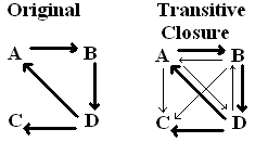
there. The transitive closure of a graph G is a graph with the
same vertices as G and an edge vw if there is a path from v to w in
G. For a small graph
you can work this out by eye easily (with or without a special
algorithm). The book's initial example is below. The
thinner edges are the ones added to make the transitive closure.
The totally connected component ABD ends up with edges between all pairs
in both directions. Since D connected to C, all other vertices in
ABD also connect to C. In general, if any edge goes from one
totally connected component to another, then in the transitive closure,
all edges in the first totally connected component are connected to
every edge in the other totally connected component.
When the graphs get big, you cannot just do them by eye. An
obvious approach for transitive
closure is just to do a DFS from each vertex. This is useful in
some cases (see homework).
There is an easy adaptation of Floyd-Warshall works, using boolean
values aij
in place of distances, and boolean operations in place of + and
min. The initial values are just those of the adjacency
matrix. The innermost line in the algorithm becomes
aij = aij or (aik and akj )
Warshall's algorithm for transitive closure is short to write, but not
the lowest order. Interpret matrix multiplication of boolean
matrices to substitute AND for multiplication and OR for addition with
an adjacency matrix A. The identity matrix I, gives all the
vertices reachable in 0 steps (just the vertices themselves). Let M =
I + A. Then M gives all vertices reachable in 0 or 1 steps.
Consider M2. It shows all vertex pairs and
if there is a connecting path between them of length at most 2. Just consider
the meaning of the sum for the ij element of M2 = mi1*m1j + mi2*m2j +...+ min*mnj + mi1*m1j
which says there is path from i to j through vertex 1, or through 2, or
... through vertex n. All the possible paths of length at most 2
are considered. Similarly, M3 = M2
* M shows all vertex pairs with connecting path between them of
length at most 3, putting all paths of length at most two with up to
one more edge. Similarly up through Mn-1, which shows
all vertex pairs with and connecting path between them of length at
most n-1. The longest possible path between the n vertices is
n-1, so Mn-1 gives all vertices reachable from
another. Put together two algorithms: the logarithmic order
algorithm for powers, calculating Mk in terms of Mk/2, and Strassen's algorithm for matrix multiplication. Using the combination, Mn-1 can be calculated in O(nlg 7 log n) using O(log n) matrix multiplications with each matrix multiplication being O(nlg 7). The order of nlg 7 log n is less than the n3
of Warshall. Given the overhead for Strassen's algorithm, this is
only better than very simple Warshall when n is very large.
Without Strassen there is still an advantage of using matrix
methods: hardware can do 32 or more one bit boolean operations in
parallel. To be effective both the matrix and its transpose need
to be updated, reducing the gain by half.
Floyd's algorithm for shortest distance is very similar to
Warshall's, but the trick with matrix
multiplication works only for transitive closure, however, since
multiplying distances does not help at all.
Dynamic programming, general introduction
Dynamic programming is a whole approach to problem solving. Getting an intuitive and practical feel for the idea
of dynamic programming is more important than the individual
examples. You can read 8.1. For an introduction to the approaches, see fib.py. This ridiculously simple example allows the techniques to be displayed with no complications obscuring them.
All these ideas apply in more complicated cases. The central
idea is that results in the recursion "tree" are reused
a lot.
Essentially that means imagining a tree
of cases is the wrong thing to
do, since we are essentially saying the branches rejoin in a common
subproblem. More generally the dependent problems form a
DAG. To take
advantage of the DAG structure there is a trade off with time and space
usually. Keeping
extra space requirements to a minimum is an issue.
In most problems,the DAG is implicit, and connections are found by
digging into the code. To emphasize the centrality of DAG's, we
can state the problem for an explicitly given DAG, where we explore the
sequence of critical path solutions: critPathRec.py, critPathDFS.py, critPathTopo.py.
Though we did a version of the last one first, it is the
most sophisticated one, improving on the others. The recursive
version recalculates for each vertex every time it is reached, so it is
inefficient if nodes are used multiple times. The DFS version
memoizes, recording data for each node and the idea if checking if a
node is visited is checking if data still needs to be calculated, or
has already been done. The reverse topological sort avoids the
memoizing.
Dynamic Programming as a Strategy
- Tends to be used for recursive optimizations where subproblems
are
reused, and there are not too many subproblems.
- Recursion makes logical sense if the optimum/answer for subproblems
carries
over as a
part of the optimum/answer for a larger problem containing the subproblem.
- Dynamic programming is distinguished from regular recursion by
the
reuse of
subproblems. It depends on the setting up the
subproblems in a way that the space for the results of all subproblems needed at one time is small enough
to fit in the memory allocation for the problem.
- In order
to store problems there must be an easy way to specify the parameters
that distinguish one subproblem from another. These parameters
are usually just the parameters that change in recursive calls in the
recursive version of the solution.
In the past classes have had a lot of trouble with this
approach. There are two quite distinct parts:
- Getting started by stating a recursive algorithm that gives the
problem-specific relation of larger problems to smaller problems.
For this part you do not need to worry about the basic dynamic
programming idea of conserving the time spent on reused problems
(except that you do want a recursive structure that does not have too
many subcases). People seem to have trouble with recursion in
general AND this is the creative part of the solution (always the main
trouble). We will spend a lot of time on this and you will need to get your recursion abilities honed!
- Given
a clearly stated relationship of larger to smaller
problems, and not having too many smaller problems total, it is a
pretty mechanical process to convert a recursive algorithm to dynamic
programming, but students still have a problem with it, I'm not sure
why. Be sure to ask questions. This is a basic ability that
I will certainly expect
of you! With little thought you can memoize. We will see
pretty standard patterns for topological orders. The most time
consuming part is keeping a secondary table to remember the optimal
choice of subproblems if you want to reproduce an optimal
sequence. This is still pretty mechanical but admittedly messy,
initially setting up pointers to the previous step, and then
traversing the optimal linked list at the end.
Work in class..... Do not look at the solutions to the next problems until we have worked out the basic ideas in class!
My code generally includes a pure recursive solution, and a dynamic
programming one with a topological order, and sometimes the longer
version allowing you to reproduce the optimal path. Before
looking at my dynamic programming solution, all
the examples are good ones for you to practice starting with the
recursive version and doing a conversion to dynamic programming,
until you are sure you clearly have the mechanics, and you can also
make sure you have the mechanics of keeping the secondary table to
reproduce the optimal path.
Consider in class the contiguous subsequence problem, finding a maximum sum: (DasGupta 6.1):
Given real numbers a1, a2, ... , an,
for each i, j, 1 <= i <= j <= n, the sequence for numbers ak,
for i <= k <= j, is a contiguous subsequence. Find the
maximum sum obtained by adding a contiguous subsequence.
What is the time for brute force? We will need to do
better....
...
Hint: Max subsequence must end somewhere. Use D(i), as the
maximal sum ending at index i, which may include no elements, and be 0,
so its minimum value is 0.
...
D(i) is either 0 or based on a sequence ending with ai. If ai is included, it never hurts to add the best sequence ending at i-1, D(i-1), since D(i-1) is at least 0. Hence
D(i) = max(0, D(i-1) + ai). See the largest
contiguous sequence sum in Python. I added a second version to keep track if the index
range of the best sequence.
Since subproblems do not get used multiple times, this is not really a
dynamic programming problem, but the recursion idea is still
important,and illustrates a generally useful point: The general
problem is
just find the largest sum, somewhere in the sequence, but we defined
D(i) with an extra condition, that the sum sequence ends at i.
This is a common distinction to consider: Possibilities:
- The subproblems can be expressed exactly like the overall
problem ( just with a smaller data set)
- The subproblem is more specific. This is often
the case when then general problem allows some data elements to be
included or not, or be the end of the part in the optimal choice or
not.... The subproblem may specify that the last element in the
partial-problem dataset IS used or IS the ending parameter in the
optimal solution. In these cases extra information needs to
be maintained (commonly a running maximum
or minimum) to produce the final answer to the more general question.
Datasets for common subproblems. The following ways of looking at
problems with one or two datasets can help you get started:
- With a single sequence of input data like a1, a2, ... , an, there are two common situations for sub problems and a less common one.
- a1, a2, ... , ai, for some i = 1, 2, ...n
- ai, ai+1, ... , aj, for some i <= j
- all subsets of the data. This is automatically
exponential in the size of the data, so it is not really good, but
sometimes the alternative is O(n!), which is much larger.
- Another possible input situation is to have two data sequences, a1, a2, ... , an, and b1, b2, ... , bm. Here the data for a subproblem is often a1, a2, ... , ai, and b1, b2, ... , bj.
- If the problem can be stated in terms of a rooted tree, subproblems often correspond to subtrees.
- Sometimes there are multiple data elements, but they make sense
to be a part of all problems, and there is a much simpler
dependency: If the problem depends on one or more positive
integer numbers parameters specific meanings (not part of a set), maybe
the dependency is just on the same problem with smaller values for
these parameters.
Of course the choice of how to set up the smaller problems depends
on
how you can relate the smaller problems to the larger problem!
That will always be problem specific. You have to
look your specific situation, and understand its ramifications.
Look at concrete examples and see what a solution to a smaller problem
had to do with a larger one. You need to gain experience working on
this! We
will see there may be multiple ways to set up relationships to smaller
problems, some impractical, others practical. For dynamic
programming to be effective, there must be a limited number of these
subproblems for two reasons:
- The overall time is related to the total number
of subproblems needing to be considered.
- If you need a table of the result of all these problems,
there is an issue of space.
Class problem solving: given a sequence of n letters or numbers,
find the longest palindrome subsequence. Unlike the last problem
or a regular palindrome, there can be gaps between elements of a
subsequence.
A palindrome subsequence of abracadabra is a b a c a b a. Another is a r a d a r a.
Develop table: sizing, initializing, filling, step by step in class!
Stub to build on basic recursive case, palindromeStub.py, using printtables.py for display:
Check later: complete
Palindrome
subsequence in Python, using printtables.py for display, with extra versions reconstructing the
palindrome, and showing off the data used for reconstruction.There are several ways to look at this problem. If you are
looking to relate it to smaller problems, what might you
consider? What smaller data set and what problem with that
dataset? Hint: Remember it may be useful to recursively
solve a problem with extra conditions, to make the recursive reasoning
easier.
Consider how to do a topological ordering in the table. Assume i
is the row and j is the column. The base cases give the main
diagonal as 1's. The 0-length intervals correspond to i=j+1 (just
below the main diagonal). The entry for (i, j) depends on table
locations (i+1, j-1), (i, j-1), (i+1, j). For instance the
position with the '?' depends on the 3 locations with D already being
filled in.
j
-----------+
1 |
01 |
01 |
i 01 D? |
01 DD |
01 |
01 |
01 |
01 |
01 |
01|
The dependency on positions down and to the left, means you want to
start as far as possible down to the left, and and work from
there. The rows are shown as an alphabetic sequence with the
direction indicated:
j
-----------+
1>>>>>>>>>z|
01 |
01 |
i 01 ... |
01 |
01>>>>e|
01>>>d|
01>>c|
01>b|
01a|
01|
My old alternate notes on two of the book's examples follow,
knapsack and sequence of matrix multiplications:
Knapsack problem
You have a knapsack which holds weight W, and you want to carry away as
much of the treasure hoard that you found as possible. There
are
n items with integer weights wi and values vi,
i
= 1, 2, ... n. What is the maximum treasure value
you can
take?
Simple example: Knapsack holds 5kg (W = 5) and there are 4
items
to choose from:
Index
|
Weight
|
Value
|
1
|
2
|
12
|
2
|
1
|
10
|
3
|
3
|
20
|
4
|
2
|
15
|
What is the brute force approach? What is the order of the
time? What is the final solution for the data above?
What is a greedy algorithm? What answer does it give for the data above?
It turns out that a very similar problem is much easier:
Suppose
all the valuables are precious metal powders, so any fraction of
an
item can be considered. Then the obvious greedy algorithm
works
to give the optimal solution. Proving this is a
reasonable
exercise.
Back to the discrete all-or-nothing case. Suppose W is way
less
than 2n. Find the outline of a dynamic
programming
solution.
. . .
Clearly it is a simpler problem with fewer items. We do not
want
to consider all 2n subsets. What else
might we
do? Add one item at a time,
so there are subproblems for the first k items, k <=
n. How can
we relate the problem for n items and max weight W to smaller problems
that do not involve the last item? How does W come
in? How
does subproblem optimality come in?
If adding wn to the knapsack provides the best
answer for
weight W, then removing the nth item must provide the best solution for
all items 1 ... n-1, for weight W-wn, so of
course the max
weight is also a parameter for the subproblems.
Let V(i, j) be the maximum value selecting among item 1, 2, ... i, if
the weight limit is j.
Then in the situation described above,
V(n,W) = vn + V(n-1, W-wn).
Complete this,
and worry about special cases.
The above equation only makes sense if (1) the nth item is
helpful (2) W-wn is nonnegative.
If we were not to include wn, V(n,
W)
would be the same as V(n-1, W). This
discussion also
applies for indices i in place of n, i = 1, 2, ...n:
. . .
Assume V(i, j) = 0 if i = 0 ( no items) or j = 0 (0 weight
limit). Then for i = 1, 2, 3, .... n, j = 1,2, ... W:
if wi > j
V(i, j) = V(i-1, j)
else
V(i, j) = max(V(i-1, j), vi
+ V(i-1, j - wi))
Clearly extra space is order of nW, since time for each entry (assuming
dependencies calculated) is O(1), total time in the order of nW
also. Note this dynamic programming algorithm is only helpful
for
sure if the order of nW is smaller than 2n.
This is
not true in general. In general this problem is hard.
With the simple sample data given above, we start with the top row and
left column of 0's, and work out one row at a time:
|
Best Value
|
| Index |
Weight |
Value |
Maximum
Weight
|
|
|
|
0
|
1
|
2
|
3
|
4
|
5
|
0
|
-
|
-
|
0
|
0
|
0
|
0
|
0
|
0
|
1
|
2
|
12
|
0
|
|
|
|
|
|
2
|
1
|
10
|
0
|
|
|
|
|
|
3
|
3
|
20
|
0
|
|
|
|
|
|
4
|
2
|
15
|
0
|
|
|
|
|
|
generating:
|
Best
Value |
| Index |
Weight |
Value |
Maximum
Weight
|
|
|
|
0
|
1
|
2
|
3
|
4
|
5
|
0
|
-
|
-
|
0
|
0
|
0
|
0
|
0
|
0
|
1
|
2
|
12
|
0
|
0
|
12
|
12
|
12
|
12
|
2
|
1
|
10
|
0
|
10
|
12
|
22
|
22
|
22
|
3
|
3
|
20
|
0
|
10
|
12
|
22
|
30
|
32
|
4
|
2
|
15
|
0
|
10
|
15
|
25
|
30
|
37
|
so the final maximum choosing between all 4 items with a
weight
limit of 5 is 37. (This was a reasonable scale to demonstrate
the
dynamic technique, though in this small case, there are more entries in
the table above than were considered by brute force!). See knapsack.py, using already referenced printtables.py for display.
Homework problem R:
Add Python code or pseudocode to print pairs (value, weight) for each
item in the optimal set, in increasing order of index. This can
be recovered from the basic table, and the lists of values and weights,
without generating a separate table, though you can generate an extra
table if you like. Hint at end.
Multiplying a sequence of varying sized matrices
Minimizing floating
point multiplication of elements when multiplying n matrices of varying
dimensions
A1 A2
A3
... An
A1
A2
A3 A4
could be
((A1
A2)A3)A4
or
((A1
A2)(A3 A4))
or
A1((A2 A3)A4)
or ...
To multiple k by m and m by n matrices need k*m*n multiplications by
the definition (ignoring Strassen and other such fancy multiplication
techniques).
Suppose the dimensions of Ak
are dk-1
by dk. The total
can be dramatically different with different orders.
If the sequence of dimensions are 30 1 40 10 25
((A1A2)A3)A4
-> 20700
(A1A2)(A3A4)
-> 41200
A1((A2A3)A4) ->
1400
One
approach is to just follow the order of computation: pick an
adjacent pair to multiple, removing one dimension. do this
recursively, testing each position. The work to multiply p by r
and r by s matrices (by definition, not Strassen) is O(prs). See multMat1.py
Time?
What if reuse results?
Another approach: How are numerical calculations generally viewed in a compiler or expression evaluator: As a tree:
*
/ \
1 *
/ \
* 4
/ \
2 3
The recursive approach to trees suggests looking at the root and
subtrees, and all subtrees that could replace a given
subtree. How can we parametrize that different
problems? Each subtree will handle a contiguous range of the
indices. Let the subproblems be f(i, j), which gives the minimum
number of multiplications for the matrices involving dimension indices
i .. j. The principal of optimality applies: The optimal
solution for a problem involves the optimal solution for
subproblems. Given the matrices for a range of dimension indices
from i through j, the question remains, where will the root of the tree
be? In other words, what will be the dimension index k, so the
left subtree comes from dimensions indices i..k, and the right subtree
comes from k..j. You need to test for each k, and take the
optimal one. Each involves a root multiplication with dk-1 * dk * dk+1 individual steps, and the ones for the smaller problems. Find the max over k of
dk-1 * dk * dk+1 + f(i, k) + f(k, j)
See the beginning of multMat2.py
(the recursive version only).
How to make a topological order?
0 entries on
diagonal are immediately known
To calculate entry at ? you depend only on the entries labeled D
---------+
0 |
0 |
0DDDD? |
0 D |
0 D |
0 D |
0D |
0 |
0
think
before looking
...
Order of calculation showing order of row order and direction in rows, similar to the palindrome example
07----->
06---->
05--->
04-->
03->
02>
01
0
MultMat2.py also uses this method, and ends with a version keeping
track for the multiplication order.
Homework Problem S:
Write an algorithm to take the last
array and
produce the correct fully parenthesized multiplication expression for the matrix multiplication, in a
form like
((1 2) (3 (4 5))) or a postfix (Reverse Polish)
notation like
1 2 * 3 4 5 * * *
For brevity and printing ease, instead of using the full subscripted matrix names as in (A1
A2), you can just use the subscripts alone as in (1 2). Hint at end.
The text covers the optimal binary search tree problem.
This is explicitly a tree problem, and immediately suggests the form of
subproblem. The algebra is more involved, until you see how it
simplifies. This section may be considered below as a
problem. It is not a really realistic solution. With the
static distribution, a hash table could be used easily.
Problems to possibly consider in class:
In all problems, besides pseudocode, analyze the order of the space and
time requirements (here and in homework).
1. Making change:
Given coin values 1 = c0 < c1 < c2 < ... < cn-1,
find the minimum number of coins needed to give amount A in change,
assuming you have a large supply of each value of coin. Note you
cannot assume US coin values, where the greedy method works, but it
does not work in general. Compare your answer to the solution dyn_coins.py. An extra elaboration would be to list the coins. (This is basically Levitin 3rd edition, section 9.1 Example 2.)
2. Determining line
splits in a paragraph with fixed width font, and penalty function for the amount
the width of all the words differs from the column width W. For
instance words of length 3, 2, 4 fit on a line of width 13. They
take up space with the intervening blanks of 3+1 + 2+1 + 4 = 11, with 2
spaces left over to give a penalty. The simple transformation is to
include the space after each work in the length of the word, and assume
the maximum width W is also one larger, so the corresponding situation
would have words of length of 4, 3, and 5 on a line of
length 14, and the extra space is 14 - (4+3+5) = 2 again. We assume this transformation.
So gives lengths w1, w2, ... , wn, and
a maximum line length W, and a penalty function f(s) for the number of
extra spaces on a line, organize a paragraph with minimum total
penalty. The assumption is that there is no penalty for a short
final line of the paragraph. An example penalty function would be
f(s) = s3. Think...
...
Brute force is ridiculous. We consider an iterative approach
building on shorter lists. We could grow the list from either
end, back or front, but it turns out that the special end penalty makes
this not be symmetric, and it is slightly easier to imagine starting
from the end and working backwards. As long as all the
words fit on one line, there is no penalty, but then.... Solution
lineBreak.py
I repeat again, the idea of transforming a recursive solution to dynamic
programming is very basic. Be sure you can do that. Besides
the homework, you can start with the recursive example solutions I give
and get the dynamic solution yourself.
- - - - -
Other possible examples:
edit distance (done in DasGupta)
fastest binary search (8.3) Python recursive only: optSearch1.py, dynamic: optSearch2.py. The latter needs printtables.py.
Longest increasing subsequence: (done in DasGupta) Given numbers a1, a2, ... , an,
find the longest strictly increasing subsequence. For example,
given 5, 2, 8, 6, 3, 6, 9, 7, some increasing subsequences are 5,
6 ,7 and 2, 3, 6, 9, which is one of the the longest ones.
DasGupta 6.3, 6,6, 6.5, 6.12, 6.21
Hints:
R: Since there are only a couple of possibilities for the reason
for
each new entry, you can just look at the table to see which place is
feeding the current entry, and work backwards as usual, though the
questions asks for the final answer to be stated forward through the
items.
S: Given the last
matrix, this is concisely stated recursively. Another chance to work on your recursion!
Next P and NP